Halden research site: geotechnical characterization of a post glacial silt

Øyvind Blaker; Roselyn Carroll; Priscilla Paniagua; Don J. DeGroot; Jean-Sebastien L'Heureux; Øyvind Blaker; Roselyn Carroll; Priscilla Paniagua; Don J. DeGroot; Jean-Sebastien L'Heureux

doi:10.3934/geosci.2019.2.184

AIMS Geosciences

2019, Volume 5, Issue 2: 184-234. doi: 10.3934/geosci.2019.2.184

Previous Article Next Article

Research article Special Issues

Halden research site: geotechnical characterization of a post glacial silt

1.
Offshore Geotechnics, Norwegian Geotechnical Institute, Sognsveien 72, N-0855 Oslo, Norway
2.
Geotechnics and Natural Hazards Trondheim, Norwegian Geotechnical Institute, Høgskoleringen 9, N-7034 Trondheim, Norway
3.
Department of Civil and Environmental Engineering, University of Massachusetts Amherst, 130 Natural Resources Road, Amherst, MA 01003, USA

Received: 04 February 2019 Accepted: 09 May 2019 Published: 20 May 2019

This paper describes the geology and geotechnical engineering properties of the Halden silt; a 10–12 m thick deposit of fjord-marine, low plasticity clayey silt. Over the last six years, the test site has been well characterized by combining the results from a number of geophysical and in situ tools, including; electrical resistivity tomography, multi-channel analysis of surface wave surveys, cone penetration testing, dissipation testing, in situ pore pressure measurements, seismic flat dilatometer testing, field vane testing, self-boring pressure meter testing, screw plate load testing and hydraulic fracture testing. The results from these investigations assist the interpretation of layering and in situ soil properties. Soil sampling and advanced laboratory testing have provided data for interpretation of geological setting and depositional history, soil fabric, strength, stiffness and hydraulic properties. However, interpretation of the stress history, based on oedometer tests and clay-based correlations to the cone penetration test, are unreliable. They contradict the depositional history, which suggests that the soil units at the site are near normally consolidated, except for some surface weathering and desiccation. Further, undrained shear strength interpretations are complex as the in situ tests are potentially influenced by partial drainage, and conventional undrained triaxial tests do not provide a unique (peak) undrained shear strength. Despite certain interpretation challenges the paper presents important reference data to assist in the interpretation and assessment of similar silts, and provide some guidance on important geotechnical properties for projects where limited design parameters are available.
- silt,
- in situ testing,
- laboratory testing,
- test site,
- site characterization,
- undrained shear strength,
- consolidation,
- stiffness
Citation: Øyvind Blaker, Roselyn Carroll, Priscilla Paniagua, Don J. DeGroot, Jean-Sebastien L'Heureux. Halden research site: geotechnical characterization of a post glacial silt[J]. AIMS Geosciences, 2019, 5(2): 184-234. doi: 10.3934/geosci.2019.2.184

Related Papers:

Abstract

This paper describes the geology and geotechnical engineering properties of the Halden silt; a 10–12 m thick deposit of fjord-marine, low plasticity clayey silt. Over the last six years, the test site has been well characterized by combining the results from a number of geophysical and in situ tools, including; electrical resistivity tomography, multi-channel analysis of surface wave surveys, cone penetration testing, dissipation testing, in situ pore pressure measurements, seismic flat dilatometer testing, field vane testing, self-boring pressure meter testing, screw plate load testing and hydraulic fracture testing. The results from these investigations assist the interpretation of layering and in situ soil properties. Soil sampling and advanced laboratory testing have provided data for interpretation of geological setting and depositional history, soil fabric, strength, stiffness and hydraulic properties. However, interpretation of the stress history, based on oedometer tests and clay-based correlations to the cone penetration test, are unreliable. They contradict the depositional history, which suggests that the soil units at the site are near normally consolidated, except for some surface weathering and desiccation. Further, undrained shear strength interpretations are complex as the in situ tests are potentially influenced by partial drainage, and conventional undrained triaxial tests do not provide a unique (peak) undrained shear strength. Despite certain interpretation challenges the paper presents important reference data to assist in the interpretation and assessment of similar silts, and provide some guidance on important geotechnical properties for projects where limited design parameters are available.

References

[1]	Lacasse S, Berre T, Lefebvre G (1985) Block sampling of sensitive clay. In: Publications Committee of XI ICSMFE, editor. Proceedings of the Eleventh International Conference on Soil Mechanics and Foundation Engineering, San Francisco, 12-16 August 1985, Rotterdam: A.A. Balkema, 887–892.
[2]	Lunne T, Long M, Forsberg CF (2003) Characterization and engineering properties of Onsøy clay. In: Tan TS, Phoon KK, Hight DW, et al., editors. Characterisation and Engineering Properties of Natural Soils, Lisse: A.A. Balkema, 395–427.
[3]	Berre T, Lunne T, Andersen KH, et al. (2007) Potential improvements of design parameters by taking block samples of soft marine Norwegian clays. Can Geotech J 44: 698–716. doi: 10.1139/t07-011
[4]	Berre T (2013) Test fill on soft plastic marine clay at Onsøy, Norway. Can Geotech J 51: 30–50.
[5]	Hight DW, Bond AJ, Legge JD (1992) Characterization of the Bothkennaar clay: an overview. Géotechnique 42: 303–347. doi: 10.1680/geot.1992.42.2.303
[6]	Ricceri G, Butterfield R (1974) An analysis of compressibility data from a deep borehole in Venice. Géotechnique 24: 175–192. doi: 10.1680/geot.1974.24.2.175
[7]	Cola S, Simonini P (2002) Mechanical behavior of silty soils of the Venice lagoon as a function of their grading characteristics. Can Geotech J 39: 879–893. doi: 10.1139/t02-037
[8]	Low HE, Maynard ML, Randolph MF, et al. (2011) Geotechnical characterisation and engineering properties of Burswood clay. Géotechnique 61: 575–591. doi: 10.1680/geot.9.P.035
[9]	Pineda JA, Suwal LP, Kelly RB, et al. (2016) Characterisation of Ballina clay. Géotechnique 66: 556–577. doi: 10.1680/jgeot.15.P.181
[10]	Kelly RB, Pineda JA, Bates L, et al. (2017) Site characterisation for the Ballina field testing facility. Géotechnique 67: 279–300. doi: 10.1680/jgeot.15.P.211
[11]	DeGroot DJ, Lutenegger AJ (2003) Geology and engineering properties of Connecticut Valley Varved Clay. In: Tan TS, Phoon KK, Hight DW et al., editors. Characterisation and Engineering Properties of Natural Soils. Lisse: A.A. Balkema, 695–724.
[12]	Lutenegger AJ, Miller GA (1994) Uplift Capacity of Small-Diameter Drilled Shafts from In Situ Tests. J Geotech Eng 120: 1362–1380. doi: 10.1061/(ASCE)0733-9410(1994)120:8(1362)
[13]	Briaud JL, Gibbens R (1999) Behavior of Five Large Spread Footings in Sand. J Geotech Geoenvironmental Eng 125: 787–796. doi: 10.1061/(ASCE)1090-0241(1999)125:9(787)
[14]	ISO (2002) Geotechnical investigation and testing-Identification and classification of soil. Part 1: Identification and description, Geneva, Switzerland: International Organization for Standardization.
[15]	Norwegian Geotechnical Society (1989) Melding 7: Veiledning for utførelse av dreietrykksondering. Rev.1 [in Norwegian], Oslo, Norway: Norwegian Geotechnical Society (NGF).
[16]	ISO (2012) Geotechnical investigation and testing-Field testing. Part 1: Electrical cone and piezocone penetration test, Geneva, Switzerland: International Organization for Standardization.
[17]	ISO (2017) Geotechnical investigation and testing-Field testing. Part 11: Flat dilatometer test, Geneva, Switzerland: International Organization for Standardization.
[18]	ISO (2012) Geotechnical investigation and testing-Field testing. Part 5: Flexible dilatometer test, Geneva, Switzerland: International Organization for Standardization.
[19]	Norwegian Geotechnical Society (2017) Melding 6: Veiledning for måling av grunnvannsstand og poretrykk. Rev. 2 [In Norwegian], Oslo, Norway: Norwegian Geotechnical Society (NGF).
[20]	Norwegian Geotechnical Society (1989) Melding 4: Veiledning for utførelse av vingeboring. Rev. 1 [in Norwegian], Oslo, Norway: Norwegian Geotechnical Society (NGF).
[21]	Bjerrum L, Andersen KH (1972) In-situ measurements of lateral pressures in clay. European Conference on Soil Mechanics and Foundation Engineering, 5 Madrid 1972 Proceedings. Madrid: Sociedad Española de Mecánica del Suelo y Cimentaciones.
[22]	Norwegian Geotechnical Society (2013) Melding 11: Veiledning for prøvetaking [In Norwegian], Oslo, Norway: Norwegian Geotechnical Society (NGF).
[23]	Lefebvre G, Poulin C (1979) A new method of sampling in sensitive clay. Can Geotech J 16: 226–233. doi: 10.1139/t79-019
[24]	Emdal A, Gylland A, Amundsen HA, et al. (2016) Mini-block sampler. Can Geotech J 53: 1235–1245. doi: 10.1139/cgj-2015-0628
[25]	Huang AB, Tai YY, Lee WF, et al. (2008) Sampling and field characterization of the silty sand in Central and Southern Taiwan. In: Huang AB, Mayne PW, editors. Geotechnical and Geophysical Site Characterization. Leiden: Taylor & Francis, 1457–1463.
[26]	Kazuo T, Kaneko S (2006) Undisturbed sampling method using thick water-soluble polymer solution Tsuchi-to-Kiso. J Jpn Geotech Soc 54: 145–148.
[27]	ISO (2014) Geotechnical investigation and testing-Laboratory testing of soil. Part 1: Determination of water conten, Geneva, Switzerland: International Organization for Standardization.
[28]	ISO (2014) Geotechnical investigation and testing-Laboratory testing of soil. Part 2: Determination of bulk density, Geneva, Switzerland: International Organization for Standardization.
[29]	ISO (2015) Geotechnical investigation and testing-Laboratory testing of soil. Part 3: Determination of particle density, Geneva, Switzerland: International Organization for Standardization.
[30]	ISO (2018) Geotechnical investigation and testing-Laboratory testing of soil. Part 12: Determination of liquid and plastic limits, Geneva, Switzerland: International Organization for Standardization.
[31]	Moum J (1965) Falling drop used for grain-size analysis of fine-grained materials. Sedimentology 5: 343–347. doi: 10.1111/j.1365-3091.1965.tb01566.x
[32]	ISO (2016) Geotechnical investigation and testing-Laboratory testing of soil. Part 4: Determination of particle size distribution, Geneva, Switzerland: International Organization for Standardization.
[33]	NS (1988) Geotechnical testing-Laboratory methods. Determination of undrained shear strength by fall-cone testing, Oslo, Norway: Standards Norway.
[34]	ISO (1994) Soil quality. Determination of the specific electrical conductivity, Geneva, Switzerland: International Organization for Standardization.
[35]	ISO (2017) Geotechnical investigation and testing-Laboratory testing of soil. Part 5: Incremental loading oedometer test, Geneva, Switzerland: International Organization for Standardization.
[36]	Sandbækken G, Berre T, Lacasse S (1986) Oedometer Testing at the Norwegian Geotechnical Institute, In: Yong RN, Townsend FC, editors, Consolidation of soils: testing and evaluation, STP 892: American Society for Testing and Materials, 329–353.
[37]	NS (1993) Geotechnical testing-Laboratory methods. Determination of one-dimensional consolidation properties by oedometer testing-Method using continuous loading, Oslo, Norway: Standards Norway.
[38]	ISO (2004) Geotechnical investigation and testing-Laboratory testing of soil. Part 11: Determination of permeability by constant and falling head, Geneva, Switzerland: International Organization for Standardization.
[39]	Wang Z, Gelius LJ, Kong FN (2009) Simultaneous core sample measurements of elastic properties and resistivity at reservoir conditions employing a modified triaxial cell-a feasibility study. Geophy Prospec 57: 1009–1026. doi: 10.1111/j.1365-2478.2009.00792.x
[40]	Berre T (1982) Triaxial Testing at the Norwegian Geotechnical Institute. Geotech Test J 5: 3–17. doi: 10.1520/GTJ10794J
[41]	ISO (2018) Geotechnical investigation and testing-Laboratory testing of soil. Part 9: Consolidated triaxial compression tests on water saturated soils, Geneva, Switzerland: International Organization for Standardization.
[42]	Bjerrum L, Landva A (1966) Direct Simple-Shear Tests on a Norwegian Quick Clay. Géotechnique 16: 1–20. doi: 10.1680/geot.1966.16.1.1
[43]	ASTM (2015) Standard Test Method for Consolidated Undrained Direct Simple Shear Testing of Fine Grain Soils, West Conshohocken, PA: ASTM International.
[44]	Dyvik R, Madshus C (1985) Lab measurements of Gmax using bender elements. In: Khosla V, editor. Advances in the Art of Testing Soils under Cyclic Conditions: Proceedings of a Session in Conjunction with the ASCE Convention in Detroit, Michigan 1985, New York: American Society of Civil Engineers, 186–196.
[45]	Sørensen R (1999) En 14C datert og dendrokronologisk kalibrert strandforskyvningskurve for søndre Østfold, Sørøst-Norge [In Norwegian], In: Selsing L, Lillehammer G, editors, Museumslandskap: artikkelsamling til Kerstin Griffin på 60-årsdagen. Stavanger: Arkeologisk museum i Stavanger, 59–70.
[46]	Klemsdal T (2002) Landformene i Østfold [In Norwegian]. Natur i Østfold 21: 7–31.
[47]	Olsen L, Sørensen E (1993) Halden 1913 II, Quaternary map, 1:50.000, with descriptions, Trondheim: Geological Survey of Norway.
[48]	Sørensen R (1979) Late Weichselian deglaciation in the Oslofjord area, south Norway. Boreas 8: 241–246.
[49]	Kenney TC (1964) Sea-Level Movements and the Geologic Histories of the Post-Glacial Marine Soils at Boston, Nicolet, Ottawa and Oslo. Géotechnique 14: 203–230. doi: 10.1680/geot.1964.14.3.203
[50]	Ostendorf DW, DeGroot DJ, Shelburne WM, et al. (2004) Hydraulic head in a clayey sand till over multiple timescales. Can Geotech J 41: 89–105. doi: 10.1139/t03-074
[51]	Norwegian Geotechnical Society (2011) Melding 2: Veiledning for symboler og definisjoner i geoteknikk-Identifisering og klassifisering av jord Rev. 2 [In Norwegian], Oslo, Norway: Norwegian Geotechnical Society (NGF).
[52]	Pettijohn FJ (1949) Sedimentary Rocks. New York: Harper and Row.
[53]	Rosenqvist IT (1975) Origin and Mineralogy Glacial and Interglacial Clays of Southern Norway. Clays Clay Miner 23: 153–159. doi: 10.1346/CCMN.1975.0230211
[54]	Solberg IL, Hansen L, Rønning JS, et al. (2012) Combined geophysical and geotechnical approach to ground investigations and hazard zonation of a quick clay area, mid Norway. Bull Eng Geol Environ 71: 119–133. doi: 10.1007/s10064-011-0363-x
[55]	Solberg IL, Rønning JS, Dalsegg E, et al. (2008) Resistivity measurements as a tool for outlining quick-clay extent and valley-fill stratigraphy: a feasibility study from Buvika, central Norway. Can Geotech J 45: 210–225. doi: 10.1139/T07-089
[56]	Hansen L, L'heureux JS, Longva O (2011) Turbiditic, clay-rich event beds in fjord-marine deposits caused by landslides in emerging clay deposits-palaeoenvironmental interpretation and role for submarine mass-wasting. Sedimentology 58: 890–915. doi: 10.1111/j.1365-3091.2010.01188.x
[57]	Norwegian Geotechnical Institute (2002) Early Soil Investigations for Fast Track Projects: Assessment of Soil Design Parameters from Index Measurements in Clays, Summary Report/Manual 521553-3, Oslo: Norwegian Geotechnical Institute.
[58]	Norwegian Geotechnical Society (2010) Melding 5: Veiledning for utførelse av trykksondering. Rev. 3 [in Norwegian], Oslo, Norway: Norwegian Geotechnical Society (NGF).
[59]	Lunne T, Strandvik SO, Kåsin K, et al. (2018) Effect of cone penetrometer type on CPTU results at a soft clay test site in Norway. In: Hicks MA, Pisanò F, Peuchen J, editors, Cone Penetration Testing 2018. Leiden: CRC Press, 417–422.
[60]	Robertson PK (1990) Soil classification using the cone penetration test. Can Geotech J 27: 151–158. doi: 10.1139/t90-014
[61]	Marchetti S (1980) In Situ Tests by Flat Dilatometer. J Geotech Eng Div 106: 299–321.
[62]	Marchetti S, Monaco P, Totani G, et al. (2006) The Flat Dilatometer Test (DMT) in soil investigations A Report by the ISSMGE Committee TC16. In: Failmezger RA, Anderson JB, editors. Proceedings from the Second International Conference on the Flat Dilatometer, Washington, DC, April 2–5, 2006, Lancaster, VA: In-Situ Soil Testing.
[63]	Marsland A, Randolph MF (1977) Comparisons of the results from pressuremeter tests and large in situ plate tests in London Clay. Géotechnique 27: 217–243. doi: 10.1680/geot.1977.27.2.217
[64]	Casagrande A (1936) The determination of the preconsolidation load and its practical significance. Proceedings of the First International Conference on Soil Mechanics and Foundation Engineering: Cambridge, MA, 22–26 June 1936. Cambridge: Graduate school of engineering, Harvard University, 60–64.
[65]	Janbu N (1963) Soil compressibility as determined by oedometer and triaxial tests. Problems of Settlements and Compressibility of Soils: Proceedings: European Conference of Soil Mechanics and Foundation Engineering, Wiesbaden, Germany, 19–25.
[66]	Pacheco Silva F (1970) A new graphical construction for determination of the pre-consolidation stress of a soil sample. Proceedings of the 4th Brazilian Conference on Soil Mechanics and Foundation Engineering, Rio de Janeiro, Brazil, 225–232.
[67]	Lunne T, Robertson PK, Powell JJM (1997) Cone penetration testing in geotechnical practice. London: Blackie Academic & Professional.
[68]	Mayne PW (2007) Cone Penetration Testing: A Synthesis of Highway Practice. NCHRP Synthesis 368. Washington, D.C.: Transportation Research Board.
[69]	Chandler RJ (1988) The In-Situ Measurement of the Undrained Shear Strength of Clays Using the Field Vane. In: Richards AF, editor. Vane Shear Strength Testing in Soils: Field and Laboratory Studies, STP 1014. West Conshohocken, PA: ASTM International, 13–32.
[70]	Mesri G, Hayat TM (1993) The coefficient of earth pressure at rest. Can Geotech J 30: 647–666. doi: 10.1139/t93-056
[71]	Palmer AC (1972) Undrained plane-strain expansion of a cylindrical cavity in clay: a simple interpretation of the pressuremeter test. Géotechnique 22: 451–457. doi: 10.1680/geot.1972.22.3.451
[72]	Wroth CP (1984) The interpretation of in situ soil tests. Géotechnique 34: 449–489. doi: 10.1680/geot.1984.34.4.449
[73]	Rix GJ, Stoke KH (1991) Correlation of Initial Tangent Modulus and Cone Resistance. In: Huang AB, editor. Calibration Chamber Testing: Proceedings of the First International Symposium (ISOCCTI), Potsdam, NY, USA, 28-29 June, 1991: Elsevier, 351–362.
[74]	Mayne PW, Rix GJ (1995) Correlations between shear wave velocity and cone tip resistance in natural clays. Soils Found 35: 107–110. doi: 10.3208/sandf1972.35.2_107
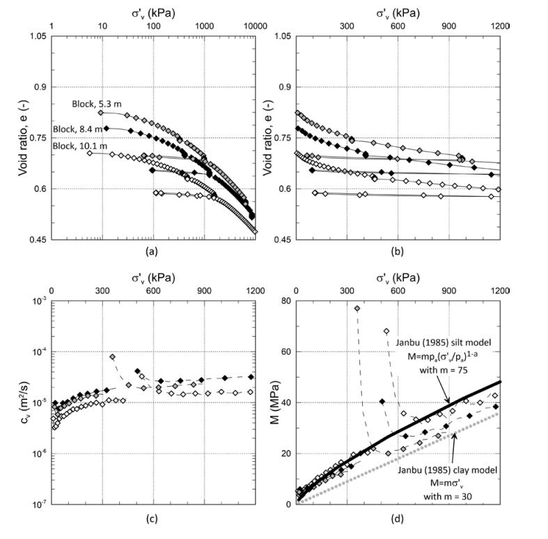
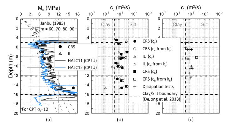
[75]	Janbu N (1985) Soil models in offshore engineering. Géotechnique 35: 241–281. doi: 10.1680/geot.1985.35.3.241
[76]	Carroll R, Long M (2017) Sample Disturbance Effects in Silt. J Geotech Geoenvironmental Eng 143: 04017061. doi: 10.1061/(ASCE)GT.1943-5606.0001749
[77]	Martins FB, Bressani LA, Coop MR, et al. (2001) Some aspects of the compressibility behaviour of a clayey sand. Can Geotech J 38: 1177–1186. doi: 10.1139/t01-048
[78]	Long M (2007) Engineering characterization of estuarine silts. Q J Eng Geol Hydrogeol 40: 147–161. doi: 10.1144/1470-9236/05-061
[79]	Long M, Gudjonsson G, Donohue S, et al. (2010) Engineering characterisation of Norwegian glaciomarine silt. Eng Geol 110: 51–65. doi: 10.1016/j.enggeo.2009.11.002
[80]	Skúlasson J (1996) Settlement investigation on Icelandic silt. In: Erlingsson S, Sigursteinsson H, editors. Interplay between geotechnics and environment : XII Nordic Geotechnical Conference, NGM-96, Reykjavik, 1996. Reykjavik: Jardtæknifélag Islands, 435–441.
[81]	DeJong JT, Jaeger RA, Boulanger RW, et al. (2013) Variable penetration rate cone testing for characterization of intermediate soils. In: Coutinho RQ, Mayne PW, editors. Geotechnical and Geophysical Site Characterization 4, Boca Raton, FL: Taylor & Francis, 25–42.
[82]	Taylor DW (1948) Fundamentals of soil mechanics. New York: J. Wiley.
[83]	Ladd CC, Weaver JS, Germaine JT, et al. (1985) Strength-Deformation Properties of Arctic Silt. In: F. Lawrence Bennett, Jerry L. Machemehl, Thelen NDW, editors. Civil Engineering in the Arctic Offshore: Conference Arctic '85, San Francisco, CA, March 25-27, 1985. New York: American Society of Civil Engineers, 820–829.
[84]	Sandven R (2003) Geotechnical properties of a natural silt deposit obtained from field and laboratory tests. In: Tan TS, Phoon KK, Hight DW et al., editors. Characterisation and Engineering Properties of Natural Soils. Lisse: A.A. Balkema, 1121–1148.
[85]	Carroll R, Paniagua López AP (2018) Variable rate of penetration and dissipation test results in a natural silty soil. In: Hicks MA, Pisanò F, Peuchen J, editors. Cone Penetration Testing 2018: Proceedings of the 4th International Symposium on Cone Penetration Testing (CPT'18), 21–22 June, 2018, Delft, The Netherlands, London: CRC Press.
[86]	Sully JP, Robertson PK, Campanella RG, et al. (1999) An approach to evaluation of field CPTU dissipation data in overconsolidated fine-grained soils. Can Geotech J 36: 369–381. doi: 10.1139/t98-105
[87]	Larsson R (1997) Investigations and load tests in silty soils. Results from a series of investigations in silty soils in Sweden. Report 54. Linköping: Swedish Geotechnical Institute, SGI, 257.
[88]	Blight GE (1968) A Note on Field Vane Testing of Silty Soils. Can Geotech J 5: 142–149. doi: 10.1139/t68-014
[89]	Gibson RE, Anderson WF (1961) In situ measurement of soil properties with the pressuremeter Civ Engi Public Work Rev 56: 615–618.
[90]	Aubeny CP, Whittle AJ, Ladd CC (2000) Effects of Disturbance on Undrained Strengths Interpreted from Pressuremeter Tests. J Geotech Geoenvironmental Eng 126: 1133–1144. doi: 10.1061/(ASCE)1090-0241(2000)126:12(1133)
[91]	Senneset K, Sandven R, Lunne T, et al. (1988) Piezocone tests in silty soils. In: de Ruiter J, editor. Penetration testing, 1988: proceedings of the First International Symposium on Penetration Testing, ISOPT-1, Orlando, 20-24 March 1988. Rotterdam, The Netherlands: A.A. Balkema, 863–870.
[92]	Brandon TL, Rose AT, Duncan JM (2006) Drained and undrained strength interpretation for low-plasticity silts. J Geotech Geoenvironmental Eng 132: 250–257. doi: 10.1061/(ASCE)1090-0241(2006)132:2(250)
[93]	Robertson PK, Campanella RG (1983) Interpretation of cone penetration tests. Part I: Sand. Can Geotech J 20: 734–745. doi: 10.1139/t83-079
[94]	Kulhawy FH, Mayne PW (1990) Manual on Estimating Soil Properties for Foundation Design, Report EL-6800, Electric Power Research Institute, Palo Alto, CA.
[95]	Janbu N, Senneset K (1974) Effective stress interpretation of in-situ static penetration tests. Proceedings of the European Symposium on Penetration Testing, ESOPT, Stockholm, June 5-7, 1974. Stockholm: National Swedish Building Research, 181–193.
[96]	Senneset K, Sandven R, Janbu N (1989) Evaluation of soil parameters from piezocone tests. Transportation Research Record 1235: 24–37.
[97]	Börgesson L (1981) Shear strength of inorganic silty soils. Proceedings of the 10th International Conference on Soil Mechanics and Foundation Engineering: 15–19 June, Stockholm,1981. Rotterdam: A.A. Balkema, 567–572.
[98]	Høeg K, Dyvik R, Sandbækken G (2000) Strength of undisturbed versus reconstituted silt and silty sand specimens. J Geotech Geoenvironmental Eng 126: 606–617. doi: 10.1061/(ASCE)1090-0241(2000)126:7(606)
[99]	Terzaghi K, Peck RB, Mesri G (1996) Soil Mechanics in Engineering Practice: John Wiley and Sons.
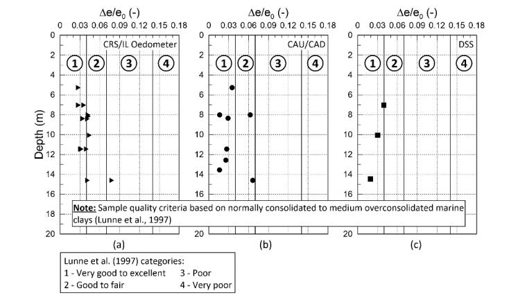
[100]	Lunne T, Berre T, Strandvik S (1997) Sample disturbance effects in soft low plastic Norwegian clay. In: Almeida M, editor. Recent Developments in Soil and Pavement Mechanics: Proceedings of the International Symposium, Rio de Janeiro, Brazil, 25–27 June 1997. Rotterdam: A.A. Balkema, 81–102.
[101]	Hight DW, Leroueil S (2003) Characterisation of soils for engineering purposes,. In: Tan TS, Phoon KK, Hight DW et al., editors. Characterisation and Engineering Properties of Natural Soils. Lisse: A.A. Balkema, 255–360.
[102]	Solhjell E, Strandvik SO, Carroll R, et al. (2017) Johan Sverdrup–Assessment of soil material behaviour and strength properties for the shallow silt layer. Offshore Site Investigation and Geotechnics, Smarter Solutions for Future Offshore Developments: Proceedings of the 8th International Conference 12-14 September 2017 Royal Geographical Society, London, UK, London: Society for Underwater Technology, 1275–1282.
[103]	Bray JD, Sancio RB, Durgunoglu T, et al. (2004) Subsurface Characterization at Ground Failure Sites in Adapazari, Turkey. J Geotech Geoenvironmental Eng 130: 673–685. doi: 10.1061/(ASCE)1090-0241(2004)130:7(673)
[104]	Arroyo M, Pineda JA, Sau N, et al. (2015) Sample quality examination in silty soils. In: Winter MG, Smith DM, Eldred PJL et al., editors. Geotechnical engineering for infrastructure and development: proceedings of the XVI European Conference on Soil Mechanics and Geotechnical Engineering, London: ICE Publishing, 2873–2878.
[105]	Bradshaw AS, Baxter CDP (2007) Sample Preparation of Silts for Liquefaction Testing. Geotech Test J 30: 324–332.
[106]	Sau N, Arroyo M, Pérez N, et al. (2014) Using CAT to obtain density maps in Sherbrooke specimens of silty soils. In: Soga K, Kumar K, Biscontin G et al., editors. Geomechanics from micro to macro: proceedings of the TC105 ISSMGE International Symposium on Geomechanics from Micro to Macro, Cambridge, UK, 1-3 September 2014. Leiden, Netherlands: CRC Press, 1153–1158.
[107]	LaRochelle P, Sarrailh J, Tavenas F, et al. (1981) Causes of sampling disturbance and design of a new sampler for sensitive soils. Can Geotech Journal 18: 52–66. doi: 10.1139/t81-006
[108]	DeJong JT, Randolph M (2012) Influence of Partial Consolidation during Cone Penetration on Estimated Soil Behavior Type and Pore Pressure Dissipation Measurements. J Geotech Geoenvironmental Eng 138: 777–788. doi: 10.1061/(ASCE)GT.1943-5606.0000646
[109]	Vesterberg B, Bertilsson R, Löfroth H (2017) Photographic feature: Monitoring of negative porewater pressure in silt slopes. Q J Eng Geol Hydrogeol 50: 245–248. doi: 10.1144/qjegh2016-083
[110]	Westerberg B, Bertilsson R, Prästings A, et al. (2014) Publication 9: Negativa portryck och stabilitet i siltslänter. Linköping: Statens Geotekniska Institut, SGI [in Swedish, with summary in English].
[111]	Clausen CJF (2003) BEAST: A computer program for limit equilibrium analysis by method of slices, Report 8302-2. Rev. 4, 24 April.

Reader Comments

Your name:*

Email:*
© 2019 the Author(s), licensee AIMS Press. This is an open access article distributed under the terms of the Creative Commons Attribution License (http://creativecommons.org/licenses/by/4.0)