The Ricci curvature and the normalized Ricci flow on the Stiefel manifolds $ \operatorname{SO}(n)/\operatorname{SO}(n-2) $

Nurlan A. Abiev; Nurlan A. Abiev

doi:10.3934/era.2025084

Electronic Research Archive

2025, Volume 33, Issue 3: 1858-1874. doi: 10.3934/era.2025084

Previous Article Next Article

Research article Special Issues

The Ricci curvature and the normalized Ricci flow on the Stiefel manifolds $ \operatorname{SO}(n)/\operatorname{SO}(n-2) $

Nurlan A. Abiev ^,

Institute of Mathematics of NAS of the Kyrgyz Republic, Bishkek 720071, Kyrgyz Republic

Received: 30 November 2024 Revised: 05 March 2025 Accepted: 12 March 2025 Published: 31 March 2025

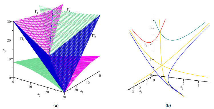
We proved that on every Stiefel manifold $ V_2\mathbb{R}^n\cong \operatorname{SO}(n)/\operatorname{SO}(n-2) $ with $ n\ge 3 $ the normalized Ricci flow preserves the positivity of the Ricci curvature of invariant Riemannian metrics with positive Ricci curvature. Moreover, the normalized Ricci flow evolves all metrics with mixed Ricci curvature into metrics with positive Ricci curvature in finite time. From the point of view of the theory of dynamical systems, we proved that for every invariant set $ \Sigma $ of the normalized Ricci flow on $ V_2\mathbb{R}^n $ defined as $ x_1^{n-2}x_2^{n-2}x_3 = c $, $ c > 0 $, there exists a smaller invariant set $ \Sigma\cap \mathscr{R}_{+} $ for every $ n\ge 3 $, where $ \mathscr{R}_{+} $ is the domain in $ \mathbb{R}_{+}^3 $ responsible for parameters $ x_1, x_2, x_3 > 0 $ of invariant Riemannian metrics on $ V_2\mathbb{R}^n $ admitting positive Ricci curvature.
- Stiefel manifold,
- Riemannian metric,
- normalized Ricci flow,
- Ricci curvature,
- dynamical system,
- invariant set,
- singular point
Citation: Nurlan A. Abiev. The Ricci curvature and the normalized Ricci flow on the Stiefel manifolds $ \operatorname{SO}(n)/\operatorname{SO}(n-2) $[J]. Electronic Research Archive, 2025, 33(3): 1858-1874. doi: 10.3934/era.2025084

Related Papers:

Abstract

We proved that on every Stiefel manifold $ V_2\mathbb{R}^n\cong \operatorname{SO}(n)/\operatorname{SO}(n-2) $ with $ n\ge 3 $ the normalized Ricci flow preserves the positivity of the Ricci curvature of invariant Riemannian metrics with positive Ricci curvature. Moreover, the normalized Ricci flow evolves all metrics with mixed Ricci curvature into metrics with positive Ricci curvature in finite time. From the point of view of the theory of dynamical systems, we proved that for every invariant set $ \Sigma $ of the normalized Ricci flow on $ V_2\mathbb{R}^n $ defined as $ x_1^{n-2}x_2^{n-2}x_3 = c $, $ c > 0 $, there exists a smaller invariant set $ \Sigma\cap \mathscr{R}_{+} $ for every $ n\ge 3 $, where $ \mathscr{R}_{+} $ is the domain in $ \mathbb{R}_{+}^3 $ responsible for parameters $ x_1, x_2, x_3 > 0 $ of invariant Riemannian metrics on $ V_2\mathbb{R}^n $ admitting positive Ricci curvature.

References

[1]	R. S. Hamilton, Three-manifolds with positive Ricci curvature, J. Differ. Geom., 17 (1982), 255–306. https://doi.org/10.4310/jdg/1214436922 doi: 10.4310/jdg/1214436922
[2]	S. Anastassiou, I. Chrysikos, The Ricci flow approach to homogeneous Einstein metrics on flag manifolds, J. Geom. Phys., 61 (2011), 1587–1600. https://doi.org/10.1016/j.geomphys.2011.03.013 doi: 10.1016/j.geomphys.2011.03.013
[3]	S. Anastassiou, I. Chrysikos, Ancient solutions of the homogeneous Ricci flow on flag manifolds, Extr. Math., 36 (2021), 99–145. https://doi.org/10.17398/2605-5686.36.1.99 doi: 10.17398/2605-5686.36.1.99
[4]	R. G. Bettiol, A. M. Krishnan, Ricci flow does not preserve positive sectional curvature in dimension four, Calc. Var. Partial Differ. Equations, 62 (2023), 13. https://doi.org/10.1007/s00526-022-02335-z doi: 10.1007/s00526-022-02335-z
[5]	M. Buzano, Ricci flow on homogeneous spaces with two isotropy summands, Ann. Global Anal. Geom., 45 (2014), 25–45. https://doi.org/10.1007/s10455-013-9386-9 doi: 10.1007/s10455-013-9386-9
[6]	A. Arvanitoyeorgos, Progress on homogeneous Einstein manifolds and some open problems, preprint, arXiv: 1605.05886.
[7]	C. Böhm, B. Wilking, Nonnegatively curved manifolds with finite fundamental groups admit metrics with positive Ricci curvature, Geom. Funct. Anal., 17 (2007), 665–681. https://doi.org/10.1007/s00039-007-0617-8 doi: 10.1007/s00039-007-0617-8
[8]	M. Cheung, N. R. Wallach, Ricci flow and curvature on the variety of flags on the two dimensional projective space over the complexes, quaternions and octonions, Proc. Am. Math. Soc., 143 (2015), 369–378. https://doi.org/10.1090/S0002-9939-2014-12241-6 doi: 10.1090/S0002-9939-2014-12241-6
[9]	N. A. Abiev, Yu. G. Nikonorov, The evolution of positively curved invariant Riemannian metrics on the Wallach spaces under the Ricci flow, Ann. Global Anal. Geom., 50 (2016), 65–84. https://doi.org/10.1007/s10455-016-9502-8 doi: 10.1007/s10455-016-9502-8
[10]	L. F. Cavenaghi, L. Grama, R. M. Martins, On the dynamics of positively curved metrics on ${\rm{SU(3)/T^2}}$ under the homogeneous Ricci flow, Matemática Contemp., 60 (2024), 3–30. http://doi.org/10.21711/231766362024/rmc602 doi: 10.21711/231766362024/rmc602
[11]	D. González-Álvaro, M. Zarei, Positive intermediate curvatures and Ricci flow, Proc. Am. Math. Soc., 152 (2024), 2637–2645. https://doi.org/10.1090/proc/16752 doi: 10.1090/proc/16752
[12]	N. Abiev, Ricci curvature and normalized Ricci flow on generalized Wallach spaces, preprint, arXiv: 2409.02570.
[13]	Yu. G. Nikonorov, Classification of generalized Wallach spaces, Geom. Dedicata, 181 (2016), 193–212. https://doi.org/10.1007/s10711-015-0119-z doi: 10.1007/s10711-015-0119-z
[14]	M. M. Kerr, New examples of homogeneous metrics, Mich. Math. J., 45 (1998), 115–134. https://doi.org/10.1307/mmj/1030132086 doi: 10.1307/mmj/1030132086
[15]	M. Statha, Invariant metrics on homogeneous spaces with equivalent isotropy summands, preprint, arXiv: 1603.06528.
[16]	M. Statha, Ricci flow on certain homogeneous spaces, Ann. Global Anal. Geom., 62 (2022), 93–127. https://doi.org/10.1007/s10455-022-09843-3 doi: 10.1007/s10455-022-09843-3
[17]	N. Abiev, On the dynamics of a three-dimensional differential system related to the normalized Ricci flow on generalized Wallach spaces, Results Math., 79 (2024), 198. https://doi.org/10.1007/s00025-024-02229-w doi: 10.1007/s00025-024-02229-w
[18]	A. Arvanitoyeorgos, Homogeneous Einstein metrics on Stiefel manifolds, Commentat. Math. Univ. Carol., 37 (1996), 627–634.
[19]	R. S. Hamilton, Non-singular solutions of the Ricci flow on three-manifolds, Commun. Anal. Geom., 7 (1999), 695–729. https://doi.org/10.4310/CAG.1999.v7.n4.a2 doi: 10.4310/CAG.1999.v7.n4.a2
[20]	J. Lauret, Ricci flow on homogeneous manifolds, Math. Z., 274 (2013), 373–403. https://doi.org/10.1007/s00209-012-1075-z doi: 10.1007/s00209-012-1075-z

Reader Comments

Your name:*

Email:*
© 2025 the Author(s), licensee AIMS Press. This is an open access article distributed under the terms of the Creative Commons Attribution License (http://creativecommons.org/licenses/by/4.0)