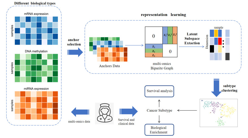
Due to the complex nature and highly heterogeneous of cancer, as well as different pathogenesis and clinical features among different cancer subtypes, it was crucial to identify cancer subtypes in cancer diagnosis, prognosis, and treatment. The rapid developments of high-throughput technologies have dramatically improved the efficiency of collecting data from various types of omics. Also, integrating multi-omics data related to cancer occurrence and progression can lead to a better understanding of cancer pathogenesis, subtype prediction, and personalized treatment options. Therefore, we proposed an efficient multi-omics bipartite graph subspace learning anchor-based clustering (MBSLC) method to identify cancer subtypes. In contrast, the bipartite graph intended to learn cluster-friendly representations. Experiments showed that the proposed MBSLC method can capture the latent spaces of multi-omics data effectively and showed superiority over other state-of-the-art methods for cancer subtype analysis. Moreover, the survival and clinical analyses further demonstrated the effectiveness of MBSLC. The code and datasets of this paper can be found in https://github.com/Julius666/MBSLC.
Citation: Shuwei Zhu, Hao Liu, Meiji Cui. Efficient multi-omics clustering with bipartite graph subspace learning for cancer subtype prediction[J]. Electronic Research Archive, 2024, 32(11): 6008-6031. doi: 10.3934/era.2024279
Due to the complex nature and highly heterogeneous of cancer, as well as different pathogenesis and clinical features among different cancer subtypes, it was crucial to identify cancer subtypes in cancer diagnosis, prognosis, and treatment. The rapid developments of high-throughput technologies have dramatically improved the efficiency of collecting data from various types of omics. Also, integrating multi-omics data related to cancer occurrence and progression can lead to a better understanding of cancer pathogenesis, subtype prediction, and personalized treatment options. Therefore, we proposed an efficient multi-omics bipartite graph subspace learning anchor-based clustering (MBSLC) method to identify cancer subtypes. In contrast, the bipartite graph intended to learn cluster-friendly representations. Experiments showed that the proposed MBSLC method can capture the latent spaces of multi-omics data effectively and showed superiority over other state-of-the-art methods for cancer subtype analysis. Moreover, the survival and clinical analyses further demonstrated the effectiveness of MBSLC. The code and datasets of this paper can be found in https://github.com/Julius666/MBSLC.

| [1] | J. Ferlay, M. Ervik, F. Lam, M. Colombet, L. Mery, M. Piñeros, et al., Global Cancer Observatory: Cancer Today, Lyon: International Agency for Research on Cancer, 2020. Available from: https://gco.iarc.fr/today. |
| [2] |
K. A. Hoadley, C. Yau, D. M. Wolf, A. D. Cherniack, D. Tamborero, S. Ng, et al., Multiplatform analysis of 12 cancer types reveals molecular classification within and across tissues of origin, Cell, 158 (2014), 929–944. https://doi.org/10.1016/j.cell.2014.06.049 doi: 10.1016/j.cell.2014.06.049

|
| [3] |
D. Sun, A. Li, B. Tang, M. Wang, Integrating genomic data and pathological images to effectively predict breast cancer clinical outcome, Comput. Methods Programs Biomed., 161 (2018), 45–53. https://doi.org/10.1016/j.cmpb.2018.04.008 doi: 10.1016/j.cmpb.2018.04.008
|
| [4] |
T. Wang, W. Shao, Z. Huang, H. Tang, J. Zhang, Z. Ding, et al., Mogonet integrates multi-omics data using graph convolutional networks allowing patient classification and biomarker identification, Nat. Commun., 12 (2021), 3445. https://doi.org/10.1038/s41467-021-23774-w doi: 10.1038/s41467-021-23774-w
|
| [5] |
J. N. Weinstein, E. A. Collisson, G. B. Mills, K. R. Shaw, B. A. Ozenberger, K. Ellrott, et al., The cancer genome atlas pan-cancer analysis project, Nat. Genet., 45 (2013), 1113–1120. https://doi.org/10.1038/ng.2764 doi: 10.1038/ng.2764
|
| [6] |
J. Zhang, R. Bajari, D. Andric, F. Gerthoffert, A. Lepsa, H. Nahal-Bose, et al., The international cancer genome consortium data portal, Nat. Biotechnol., 37 (2019), 367–369. https://doi.org/10.1038/s41587-019-0055-9 doi: 10.1038/s41587-019-0055-9
|
| [7] |
X. Liu, Y. Tao, Z. Cai, P. Bao, H. Ma, K. Li, et al., Pathformer: a biological pathway informed transformer for disease diagnosis and prognosis using multi-omics data, Bioinformatics, 40 (2024), btae316. https://doi.org/10.1093/bioinformatics/btae316 doi: 10.1093/bioinformatics/btae316
|
| [8] |
J. Zhao, B. Zhao, X. Song, C. Lyu, W. Chen, Y. Xiong, et al., Subtype-DCC: decoupled contrastive clustering method for cancer subtype identification based on multi-omics data, Briefings Bioinf., 24 (2023), bbad025. https://doi.org/10.1093/bib/bbad025 doi: 10.1093/bib/bbad025
|
| [9] |
S. Zhu, W. Wang, W. Fang, M. Cui, Autoencoder-assisted latent representation learning for survival prediction and multi-view clustering on multi-omics cancer subtyping, Math. Biosci. Eng., 20 (2023), 21098–21119. https://doi.org/10.3934/mbe.2023933 doi: 10.3934/mbe.2023933
|
| [10] |
X. Ye, T. Shi, Y. Cui, T. Sakurai, Interactive gene identification for cancer subtyping based on multi-omics clustering, Methods, 211 (2023), 61–67. https://doi.org/10.1016/j.ymeth.2023.02.005 doi: 10.1016/j.ymeth.2023.02.005
|
| [11] |
M. Lovino, V. Randazzo, G. Ciravegna, P. Barbiero, E. Ficarra, G. Cirrincione, A survey on data integration for multi-omics sample clustering, Neurocomputing, 488 (2022), 494–508. https://doi.org/10.1016/j.neucom.2021.11.094 doi: 10.1016/j.neucom.2021.11.094
|
| [12] |
D. Wu, D. Wang, M. Q. Zhang, J. Gu, Fast dimension reduction and integrative clustering of multi-omics data using low-rank approximation: application to cancer molecular classification, BMC Genomics, 16 (2015), 1–10. https://doi.org/10.1186/s12864-015-2223-8 doi: 10.1186/s12864-015-2223-8
|
| [13] |
X. Ye, W. Zhang, Y. Futamura, T. Sakurai, Detecting interactive gene groups for single-cell rna-seq data based on co-expression network analysis and subgraph learning, Cells, 9 (2020), 1938. https://doi.org/10.3390/cells9091938 doi: 10.3390/cells9091938
|
| [14] |
S. Zhu, L. Xu, Many-objective fuzzy centroids clustering algorithm for categorical data, Expert Syst. Appl., 96 (2018), 230–248. https://doi.org/10.1016/j.eswa.2017.12.013 doi: 10.1016/j.eswa.2017.12.013
|
| [15] |
S. Zhu, L. Xu, E. D. Goodman, Hierarchical topology-based cluster representation for scalable evolutionary multiobjective clustering, IEEE Trans. Cybern., 52 (2022), 9846–9860. https://doi.org/10.1109/TCYB.2021.3081988 doi: 10.1109/TCYB.2021.3081988
|
| [16] |
B. Yang, T. T. Xin, S. M. Pang, M. Wang, Y. J. Wang, Deep subspace mutual learning for cancer subtypes prediction, Bioinformatics, 37 (2021), 3715–3722. https://doi.org/10.1093/bioinformatics/btab625 doi: 10.1093/bioinformatics/btab625
|
| [17] |
J. M. Nigro, A. Misra, L. Zhang, I. Smirnov, H. Colman, C. Griffin, et al., Integrated array-comparative genomic hybridization and expression array profiles identify clinically relevant molecular subtypes of glioblastoma, Cancer Res., 65 (2005), 1678–1686. https://doi.org/10.1158/0008-5472.CAN-04-2921 doi: 10.1158/0008-5472.CAN-04-2921
|
| [18] |
B. Wang, A. M. Mezlini, F. Demir, M. Fiume, Z. Tu, M. Brudno, et al., Similarity network fusion for aggregating data types on a genomic scale, Nat. Methods, 11 (2014), 333–337. https://doi.org/10.1038/nmeth.2810 doi: 10.1038/nmeth.2810
|
| [19] |
N. K. Speicher, N. Pfeifer, Integrating different data types by regularized unsupervised multiple kernel learning with application to cancer subtype discovery, Bioinformatics, 31 (2015), i268–i275. https://doi.org/10.1093/bioinformatics/btv244 doi: 10.1093/bioinformatics/btv244
|
| [20] |
C. Liang, M. Shang, J. Luo, Cancer subtype identification by consensus guided graph autoencoders, Bioinformatics, 37 (2021), 4779–4786. https://doi.org/10.1093/bioinformatics/btab535 doi: 10.1093/bioinformatics/btab535
|
| [21] |
N. Rappoport, R. Shamir, NEMO: cancer subtyping by integration of partial multi-omic data, Bioinformatics, 35 (2019), 3348–3356. https://doi.org/10.1093/bioinformatics/btz058 doi: 10.1093/bioinformatics/btz058
|
| [22] |
W. Wang, X. Zhang, D. Q. Dai, Defusion: a denoised network regularization framework for multi-omics integration, Briefings Bioinf., 22 (2021), bbab057. https://doi.org/10.1093/bib/bbab057 doi: 10.1093/bib/bbab057
|
| [23] |
R. Argelaguet, B. Velten, D. Arnol, S. Dietrich, T. Zenz, J. C. Marioni, et al., Multi-omics factor analysis—a framework for unsupervised integration of multi-omics data sets, Mol. Syst. Biol., 14 (2018), e8124. https://doi.org/10.15252/msb.20178124 doi: 10.15252/msb.20178124
|
| [24] |
B. Yang, T. T. Xin, S. M. Pang, M. Wang, Y. J. Wang, Deep subspace mutual learning for cancer subtypes prediction, Bioinformatics, 37 (2021), 3715–3722. https://doi.org/10.1093/bioinformatics/btab625 doi: 10.1093/bioinformatics/btab625
|
| [25] |
X. Ye, Y. Shang, T. Shi, W. Zhang, T. Sakurai, Multi-omics clustering for cancer subtyping based on latent subspace learning, Comput. Biol. Med., 164 (2023), 107223. https://doi.org/10.1016/j.compbiomed.2023.107223 doi: 10.1016/j.compbiomed.2023.107223
|
| [26] |
Z. Chen, X. J. Wu, T. Xu, J. Kittler, Fast self-guided multi-view subspace clustering, IEEE Trans. Image Process., 32 (2023), 6514–6525. https://doi.org/10.1109/TIP.2023.3261746 doi: 10.1109/TIP.2023.3261746
|
| [27] |
K. K. Sharma, A. Seal, Multi-view spectral clustering for uncertain objects, Inf. Sci., 547 (2021), 723–745. https://doi.org/10.1016/j.ins.2020.08.080 doi: 10.1016/j.ins.2020.08.080
|
| [28] |
H. Xu, X. Zhang, W. Xia, Q. Gao, X. Gao, Low-rank tensor constrained co-regularized multi-view spectral clustering, Neural Networks, 132 (2020), 245–252. https://doi.org/10.1016/j.neunet.2020.08.019 doi: 10.1016/j.neunet.2020.08.019
|
| [29] |
Z. Huang, J. T. Zhou, H. Zhu, C. Zhang, J. Lv, X. Peng, Deep spectral representation learning from multi-view data, IEEE Trans. Image Process., 30 (2021), 5352–5362. https://doi.org/10.1109/TIP.2021.3083072 doi: 10.1109/TIP.2021.3083072
|
| [30] |
X. Cai, D. Huang, G. Y. Zhang, C. D. Wang, Seeking commonness and inconsistencies: A jointly smoothed approach to multi-view subspace clustering, Inf. Fusion, 91 (2023), 364–375. https://doi.org/10.1016/j.inffus.2022.10.020 doi: 10.1016/j.inffus.2022.10.020
|
| [31] |
R. Vidal, Subspace clustering, IEEE Signal Process Mag., 28 (2011), 52–68. https://doi.org/10.1109/MSP.2010.939739 doi: 10.1109/MSP.2010.939739
|
| [32] | G. Guo, H. Wang, D. Bell, Y. Bi, K. Greer, KNN model-based approach in classification, in On The Move to Meaningful Internet Systems 2003: CoopIS, DOA, and ODBASE: OTM Confederated International Conferences, CoopIS, DOA, and ODBASE 2003, Catania, Sicily, Italy, November 3–7, 2003. Proceedings, Springer, (2003), 986–996. https://doi.org/10.1007/b94348 |
| [33] | Z. Kang, W. Zhou, Z. Zhao, J. Shao, M. Han, Z. Xu, Large-scale multi-view subspace clustering in linear time, in Proceedings of the AAAI Conference on Artificial Intelligence, 34 (2020), 4412–4419. https://doi.org/10.1609/aaai.v34i04.5867 |
| [34] | Y. Li, F. Nie, H. Huang, J. Huang, Large-scale multi-view spectral clustering via bipartite graph, in Proceedings of the AAAI Conference on Artificial Intelligence, 29 (2015), 2750–2756. https://doi.org/10.1609/aaai.v29i1.9598 |
| [35] |
S. Zhu, L. Xu, E. D. Goodman, Evolutionary multi-objective automatic clustering enhanced with quality metrics and ensemble strategy, Knowledge-Based Syst., 188 (2020), 1–21. https://doi.org/10.1016/j.knosys.2019.105018 doi: 10.1016/j.knosys.2019.105018
|
| [36] |
K. Krishna, M. N. Murty, Genetic k-means algorithm, IEEE Trans. Syst. Man Cybern. Part B Cybern., 29 (1999), 433–439. https://doi.org/10.1109/3477.764879 doi: 10.1109/3477.764879
|
| [37] |
W. Xia, Q. Gao, Q. Wang, X. Gao, C. Ding, D. Tao, Tensorized bipartite graph learning for multi-view clustering, IEEE Trans. Pattern Anal. Mach. Intell., 45 (2022), 5187–5202. https://doi.org/10.1109/TPAMI.2022.3187976 doi: 10.1109/TPAMI.2022.3187976
|
| [38] | I. Jolliffe, Principal component analysis, in Encyclopedia of Statistics in Behavioral Science, John Wiley and Sons Ltd, New York, (2005), 1580–1584. https://doi.org/10.1002/9781118445112 |
| [39] |
C. R. John, D. Watson, M. R. Barnes, C. Pitzalis, M. J. Lewis, Spectrum: fast density-aware spectral clustering for single and multi-omic data, Bioinformatics, 36 (2020), 1159–1166. https://doi.org/10.1101/636639 doi: 10.1101/636639
|
| [40] |
T. Xu, T. D. Le, L. Liu, N. Su, R. Wang, B. Sun, et al., CancerSubtypes: an R/Bioconductor package for molecular cancer subtype identification, validation and visualization, Bioinformatics, 33 (2017), 3131–3133. https://doi.org/10.1093/bioinformatics/btx378 doi: 10.1093/bioinformatics/btx378
|
| [41] |
D. Leng, L. Zheng, Y. Wen, Y. Zhang, L. Wu, J. Wang, et al., A benchmark study of deep learning-based multi-omics data fusion methods for cancer, Genome Biol., 23 (2022), 171. https://doi.org/10.1186/s13059-022-02739-2 doi: 10.1186/s13059-022-02739-2
|
| [42] |
F. E. Harrell, R. M. Califf, D. B. Pryor, K. L. Lee, R. A. Rosati, Evaluating the yield of medical tests, JAMA, 247 (1982), 2543–2546. https://doi.org/10.1001/jama.1982.03320430047030 doi: 10.1001/jama.1982.03320430047030
|
| [43] | L. Van der Maaten, G. Hinton, Visualizing data using t-SNE, J. Mach. Learn. Res., 9 (2008), 11. |
| [44] |
C. Zhou, E. Martinez, D. Di Marcantonio, N. Solanki-Patel, T. Aghayev, S. Peri, et al., JUN is a key transcriptional regulator of the unfolded protein response in acute myeloid leukemia, Leukemia, 31 (2017), 1196–1205. https://doi.org/10.1038/leu.2016.329 doi: 10.1038/leu.2016.329
|
| [45] | G. H. Su, W. Hilgers, M. C. Shekher, D. J. Tang, C. J. Yeo, R. H. Hruban, et al., Alterations in pancreatic, biliary, and breast carcinomas support MKK4 as a genetically targeted tumor suppressor gene, Cancer Res., 58 (1998), 2339–2342. |


Figures(12) / Tables(6)
Shuwei Zhu, Hao Liu, Meiji Cui. Efficient multi-omics clustering with bipartite graph subspace learning for cancer subtype prediction[J]. Electronic Research Archive, 2024, 32(11): 6008-6031. doi: 10.3934/era.2024279


 DownLoad: