Parkinson's disease is associated with bursting of the thalamic (TC) neuron, which receives the inhibitory synaptic current of the basal ganglia composed of multiple nuclei; deep brain stimulation (DBS) applied to the basal ganglia can eliminate the bursting to recover to the normal state. In this paper, the complex nonlinear dynamics for the appearance and disappearance of the bursting are obtained in a widely used theoretical model of a neuronal network. First, through a bifurcation analysis, isolated TC neurons exhibit paradoxical bursting induced from the resting state by enhanced inhibitory effect, which is different from the common view that the enhanced inhibitory effect should suppress the electrical behaviors. Second, the mechanism for the appearance of bursting is obtained by analyzing the electrical activities of the basal ganglia. The inhibitory synaptic current from the external segment of the globus pallidus (GPe) induces a reduced firing rate of the subthalamic nucleus (STN); then, an excitatory synaptic current from the STN induces the bursting behaviors of the GPe. The excitatory current of STN neurons and the inhibitory current of the GPe cause bursting behaviors of the internal segment of the globus pallidus (GPi), thus resulting in an enhanced inhibition from the GPi to the TC, which can induce the paradoxical bursting similar to the isolated TC neurons. Third, the cause for the disappearance of paradoxical bursting is acquired.The high frequency pulses of DBS induces enhanced firing activity of the STN and GPe neurons and enhanced inhibitory synaptic current from the GPe to the GPi, resulting in a reduced inhibitory effect from the GPi to the TC, which can eliminate the paradoxical bursting. Finally, the fast-slow dynamics of the paradoxical bursting of isolated TC neurons are acquired, which is related to the saddle-node and saddle-homoclinic orbit bifurcations of the fast subsystem of the TC neuron model. The results provide theoretical support for understanding the mechanism of Parkinson's disease and treatment methods such as DBS.
Citation: Hui Zhou, Bo Lu, Huaguang Gu, Xianjun Wang, Yifan Liu. Complex nonlinear dynamics of bursting of thalamic neurons related to Parkinson's disease[J]. Electronic Research Archive, 2024, 32(1): 109-133. doi: 10.3934/era.2024006
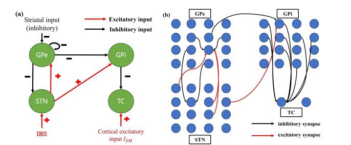
Parkinson's disease is associated with bursting of the thalamic (TC) neuron, which receives the inhibitory synaptic current of the basal ganglia composed of multiple nuclei; deep brain stimulation (DBS) applied to the basal ganglia can eliminate the bursting to recover to the normal state. In this paper, the complex nonlinear dynamics for the appearance and disappearance of the bursting are obtained in a widely used theoretical model of a neuronal network. First, through a bifurcation analysis, isolated TC neurons exhibit paradoxical bursting induced from the resting state by enhanced inhibitory effect, which is different from the common view that the enhanced inhibitory effect should suppress the electrical behaviors. Second, the mechanism for the appearance of bursting is obtained by analyzing the electrical activities of the basal ganglia. The inhibitory synaptic current from the external segment of the globus pallidus (GPe) induces a reduced firing rate of the subthalamic nucleus (STN); then, an excitatory synaptic current from the STN induces the bursting behaviors of the GPe. The excitatory current of STN neurons and the inhibitory current of the GPe cause bursting behaviors of the internal segment of the globus pallidus (GPi), thus resulting in an enhanced inhibition from the GPi to the TC, which can induce the paradoxical bursting similar to the isolated TC neurons. Third, the cause for the disappearance of paradoxical bursting is acquired.The high frequency pulses of DBS induces enhanced firing activity of the STN and GPe neurons and enhanced inhibitory synaptic current from the GPe to the GPi, resulting in a reduced inhibitory effect from the GPi to the TC, which can eliminate the paradoxical bursting. Finally, the fast-slow dynamics of the paradoxical bursting of isolated TC neurons are acquired, which is related to the saddle-node and saddle-homoclinic orbit bifurcations of the fast subsystem of the TC neuron model. The results provide theoretical support for understanding the mechanism of Parkinson's disease and treatment methods such as DBS.

| [1] |
M. M. McGregor, A. B. Nelson, Circuit mechanisms of Parkinson's disease, Neuron, 101 (2019), 1042–1056. https://doi.org/10.1016/j.neuron.2019.03.004 doi: 10.1016/j.neuron.2019.03.004

|
| [2] |
M. M. McGregor, A. B. Nelson, Directly to the point: dopamine persistently enhances excitability of direct pathway striatal neurons, Neuron, 106 (2020), 201–203. https://doi.org/10.1016/j.neuron.2020.04.005 doi: 10.1016/j.neuron.2020.04.005
|
| [3] |
P. Zhao, B. Zhang, Y. Xiao, P. Kong, F. Sun, Therapeutic effect observation of selegiline hydrochloride in early stage of Parkinson's disease, J. Clin. Neurol., 18 (2005), 306–307. https://doi.org/10.3969/j.issn.1004-1648.2005.04.023 doi: 10.3969/j.issn.1004-1648.2005.04.023
|
| [4] |
M. Jakobs, D. J. Lee, A. M. Lozano, Modifying the progression of Alzheimer's and Parkinson's disease with deep brain stimulation, Neuropharmacology, 171 (2020), 107860. https://doi.org/10.1016/j.neuropharm.2019.107860 doi: 10.1016/j.neuropharm.2019.107860
|
| [5] |
J. Kim, Y. Kim, R. Nakajima, Inhibitory basal ganglia inputs induce excitatory motor signals in the thalamus, Neuron, 95 (2017), 1181–1196. https://doi.org/10.1016/j.neuron.2017.08.028 doi: 10.1016/j.neuron.2017.08.028
|
| [6] |
Y. Yu, F. Han, Q. Wang, Q. Wang, Model-based optogenetic stimulation to regulate beta oscillations in Parkinsonian neural networks, Cognit. Neurodyn., 16 (2022), 667–681. https://doi.org/10.1007/s11571-021-09729-3 doi: 10.1007/s11571-021-09729-3
|
| [7] |
Y. Yu, X. Wang, Q. Wang, Q. Wang, A review of computational modeling and deep brain stimulation: applications to Parkinson's disease, Appl. Math. Mech., 41 (2020), 1747–1768. https://doi.org/10.1007/s10483-020-2689-9 doi: 10.1007/s10483-020-2689-9
|
| [8] |
D. Terman, J. E. Rubin, A. C. Yew, C. J. Wilson, Activity patterns in a model for the subthalamopallidal network of the basal ganglia, J. Neurosci., 22 (2002), 2963–2976. https://doi.org/10.1523/JNEUROSCI.22-07-02963.2002 doi: 10.1523/JNEUROSCI.22-07-02963.2002
|
| [9] |
J. E. Rubin, D. Terman, High frequency stimulation of the subthalamic nucleus eliminates pathological thalamic rhythmicity in a computational model, J. Comput. Neurosci., 16 (2004), 211–235. https://doi.org/10.1023/B:JCNS.0000025686.47117.67 doi: 10.1023/B:JCNS.0000025686.47117.67
|
| [10] |
R. Q. So, A. R. Kent, W. M. Grill, Relative contributions of local cell and passing fiber activation and silencing to changes in thalamic fidelity during deep brain stimulation and lesioning: a computational modeling study, J. Comput. Neurosci., 32 (2012), 499–519. https://doi.org/10.1007/s10827-011-0366-4 doi: 10.1007/s10827-011-0366-4
|
| [11] |
Y. Yu, F. Han, Q. Wang, Exploring phase-amplitude coupling from primary motor cortex-basal ganglia-thalamus network model, Neural Networks, 153 (2022), 130–141. https://doi.org/10.1016/j.neunet.2022.05.027 doi: 10.1016/j.neunet.2022.05.027
|
| [12] |
H. A. Braun, H. Wissing, K. Schafer, M. C. Hirsch, Oscillation and noise determine signal transduction in shark multimodal sensory cells, Nature, 367 (1994), 270–273. https://doi.org/10.1038/367270a0 doi: 10.1038/367270a0
|
| [13] |
H. Gu, B. Pan, G. Chen, L. Duan, Biological experimental demonstration of bifurcations from bursting to spiking predicted by theoretical models, Nonlinear Dyn., 78 (2014), 391–407. https://doi.org/10.1007/s11071-014-1447-5 doi: 10.1007/s11071-014-1447-5
|
| [14] |
H. Gu, B. Pan, Identification of neural firing patterns, frequency and temporal coding mechanisms in individual aortic baroreceptors, Front. Comput. Neurosci., 9 (2015). https://doi.org/10.3389/fncom.2015.00108 doi: 10.3389/fncom.2015.00108
|
| [15] |
Y. Yang, Y. Cui, K. Sang, Y. Dong, Z. Ni, S. Ma, et al., Ketamine blocks bursting in the lateral habenula to rapidly relieve depression, Nature, 554 (2018), 317–322. https://doi.org/10.1038/nature25509 doi: 10.1038/nature25509
|
| [16] |
E. M. Izhikevich, Neural excitability, spiking and bursting, Int. J. Bifurcation Chaos, 10 (2000), 1171–1266. https://doi.org/10.1142/S0218127400000840 doi: 10.1142/S0218127400000840
|
| [17] |
L. Duan, W. Liang, W. Ji, H. Xi, Bifurcation patterns of bursting within pre-Bötzinger complex and their control, Int. J. Bifurcation Chaos, 30 (2020), 2050192. https://doi.org/10.1142/S0218127420501928 doi: 10.1142/S0218127420501928
|
| [18] |
Y. Jiang, B. Lu, W. Zhang, H. Gu, Fast autaptic feedback induced-paradoxical changes of mixed-mode bursting and bifurcation mechanism, Acta Phys. Sin., 70 (2021), 170501. https://doi.org/10.7498/aps.70.20210208 doi: 10.7498/aps.70.20210208
|
| [19] |
Y. Liang, B. Lu, H. Gu, Analysis to dynamics of complex electrical activities in Wilson model of brain neocortical neuron using fast-slow variable dissection with two slow variables, Acta Phys. Sin., 71 (2022), 230502. https://doi.org/10.7498/aps.71.20221416 doi: 10.7498/aps.71.20221416
|
| [20] |
B. Lu, H. Gu, X. Wang, H. Hua, Paradoxical enhancement of neuronal bursting response to negative feedback of autapse and the nonlinear mechanism, Chaos, Solitons Fractals, 145 (2021), 110817. https://doi.org/10.1016/j.chaos.2021.110817 doi: 10.1016/j.chaos.2021.110817
|
| [21] |
A. Destexhe, M. Neubig, D. Ulrich, J. Huguenard, Dendritic low-threshold calcium currents in thalamic relay cells, J. Neurosci., 18 (1998), 3574–3588. https://doi.org/10.1523/JNEUROSCI.18-10-03574.1998 doi: 10.1523/JNEUROSCI.18-10-03574.1998
|
| [22] |
J. M. Goaillard, A. L. Taylor, S. R. Pulver, E. Marder, Slow and persistent postinhibitory rebound acts as an intrinsic short-term memory mechanism, Phys. Rev. Lett., 30 (2010), 4687–4692. https://doi.org/10.1523/JNEUROSCI.2998-09.2010 doi: 10.1523/JNEUROSCI.2998-09.2010
|
| [23] |
R. Felix, A. Fridberger, S. Leijon, A. S. Berrebi, Sound rhythms are encoded by postinhibitory rebound spiking in the superior paraolivary nucleus, J. Neurosci., 31 (2011), 12566–12578. https://doi.org/10.1523/JNEUROSCI.2450-11.2011 doi: 10.1523/JNEUROSCI.2450-11.2011
|
| [24] |
K. Ma, H. Gu, Y. Jia, The neuronal and synaptic dynamics underlying post-inhibitory rebound burst related to major depressive disorder in the lateral habenula neuron model, Cognit. Neurodyn., 2023 (2023). https://doi.org/10.1007/s11571-023-09960-0 doi: 10.1007/s11571-023-09960-0
|
| [25] |
W. M. Howe, P. J. Kenny, Burst firing sets the stage for depression, Nature, 554 (2018), 304–305. https://doi.org/10.1038/d41586-018-01588-z doi: 10.1038/d41586-018-01588-z
|
| [26] |
K. Chen, L. Aradi, N. Thon, M. Ahmadi, Persistently modified h-channels after complex febrile seizures convert the seizure-induced enhancement of inhibition to hyperexcitability, Nat. Med., 7 (2001), 331–337. https://doi.org/10.1038/85480 doi: 10.1038/85480
|
| [27] |
M. Chang, J. A. Dian, S. Dufour, L. Wang, H. M. Chameh, M. Ramani, et al., Brief activation of GABAergic interneurons initiates the transition to ictal events through post-inhibitory rebound excitation, Neurobiol. Dis., 109 (2018), 102–116. https://doi.org/10.1016/j.nbd.2017.10.007 doi: 10.1016/j.nbd.2017.10.007
|
| [28] |
A. Destexhe, T. Bal, D. A. Mccormick, T. J. Sejnowski, Ionic mechanisms underlying synchronized oscillations and propagating waves in a model of ferret thalamic slices, J. Neurophysiol., 76 (1996), 2049–2070. https://doi.org/10.1152/jn.1996.76.3.2049 doi: 10.1152/jn.1996.76.3.2049
|
| [29] |
A. Destexhe, T. J. Sejnowski, The initiation of bursts in thalamic neurons and the cortical control of thalamic sensitivity, Phil. Trans. R. Soc. B, 357 (2002), 1649–1657. https://doi.org/10.1098/rstb.2002.1154 doi: 10.1098/rstb.2002.1154
|
| [30] |
B. Cao, L. Guan, H. Gu, Bifurcation mechanism of not increase but decrease of spike number within a neural burst induced by excitatory effect, Acta Phys. Sin., 67 (2018), 240502. https://doi.org/10.7498/aps.67.20181675 doi: 10.7498/aps.67.20181675
|
| [31] |
H. Hua, B. Lu, H. Gu, Nonlinear mechanism of excitatory autapse-induced reduction or enhancement of firing frequency of neuronal Bursting, Acta Phys. Sin., 69 (2020), 090502. https://doi.org/10.7498/aps.69.20191709 doi: 10.7498/aps.69.20191709
|
| [32] |
Y. Yang, Y. Li, H. Gu, Nonlinear mechanisms for opposite responses of bursting activities induced by inhibitory autapse with fast and slow time scale, Nonlinear Dyn., 111 (2023), 7751–7772. https://doi.org/10.1007/s11071-023-08229-9 doi: 10.1007/s11071-023-08229-9
|
| [33] |
X. Wang, H. Gu. Y. Jia, Nonlinear mechanism for enhanced and reduced bursting activity respectively induced by fast and slow excitatory autapse, Chaos, Solitons Fractals, 116 (2023), 112904. https://doi.org/10.1016/j.chaos.2022.112904 doi: 10.1016/j.chaos.2022.112904
|
| [34] |
X. Wang, H. Gu, Post inhibitory rebound spike related to nearly vertical nullcline for small homoclinic and saddle-node bifurcations, Electron. Res. Arch., 30 (2022), 459–480. https://doi.org/10.3934/era.2022024 doi: 10.3934/era.2022024
|
| [35] |
B. Lu, S. Liu, X. Liu, X. Jiang, Bifurcation and spike adding transition in Chay-Keizer Model, Int. J. Bifurcation Chaos, 26 (2016), 1650090. https://doi.org/10.1142/S0218127416500905 doi: 10.1142/S0218127416500905
|
| [36] |
B. Lu, X. Jiang, Reduced and bifurcation analysis of intrinsically bursting neuron model, Electron. Res. Arch., 31 (2023), 5928–5945. https://doi.org/10.3934/era.2023301 doi: 10.3934/era.2023301
|
| [37] | E. M. Izhikevich, Dynamical Systems in Neuroscience: The Geometry of Excitability and Bursting, MIT Press, 2006. https://doi.org/10.7551/mitpress/2526.001.0001 |
| [38] |
A. Dhooge, W. Govaerts, Y. A. Kuznetsov, MATCONT: a Matlab package for numerical bifurcation analysis of ODEs, ACM Trans. Math. Software, 29 (2003), 141–164. http://dx.doi.org/10.1145/779359.779362 doi: 10.1145/779359.779362
|
| [39] |
M. E. Rush, J. Rinzel, Analysis of bursting in a thalamic neuron model, Biol. Cybern., 71 (1994), 281–291. https://doi.org/10.1007/BF00239616 doi: 10.1007/BF00239616
|
| [40] |
S. Li, G. W. Arbuthnott, M. J. Jutras, J. A. Goldberg, D. Jaeger, Resonant antidromic cortical circuit activation as a consequence of high-frequency subthalamic deep-brain stimulation, J. Neurophysiol., 98 (2007), 3525–3527. https://doi.org/10.1152/jn.00808.2007 doi: 10.1152/jn.00808.2007
|
| [41] |
X. Shi, Z. Zhang, Multiple-site deep brain stimulation with delayed rectangular waveforms for Parkinson's disease, Electron. Res. Arch., 29 (2021), 3471–3487. https://doi.org/10.3934/era.2021048 doi: 10.3934/era.2021048
|
| [42] |
D. A. McCormick, H. R. Feeser, Functional implications of burst firing and single spike activity in lateral geniculate relay neurons, Neuroscience, 39 (1990), 103–113. https://doi.org/10.1016/0306-4522(90)90225-s doi: 10.1016/0306-4522(90)90225-s
|
| [43] |
X. Shi, D. Du, Y. Wang, Interaction of indirect and hyperdirect pathways on synchrony and tremor-related oscillation in the basal ganglia, Neural Plast., 2021 (2021), 6640105. https://doi.org/10.1155/2021/6640105 doi: 10.1155/2021/6640105
|
| [44] |
E. Cheong, Y. Zheng, K. Lee, H. S. Shin, Deletion of phospholipase C $\beta$ 4 in thalamocortical relay nucleus leads to absence seizures, PNAS, 106 (2009), 21912–21917. https://doi.org/10.1073/pnas.0912204106 doi: 10.1073/pnas.0912204106
|
| [45] |
M. Wang, J. Wang, Dynamical balance between excitation and inhibition of feedback neural circuit via inhibitory synaptic plasticity, Acta Phys. Sin., 64 (2015), 108701. https://doi.org/10.7498/aps.64.108701 doi: 10.7498/aps.64.108701
|
| [46] |
A. Lahiri, M. Bevan, Dopaminergic transmission rapidly and persistently enhances excitability of D1 receptor-expressing striatal projection neurons, Neuron, 106 (2020), 227–290. https://doi.org/10.1016/j.neuron.2020.01.028 doi: 10.1016/j.neuron.2020.01.028
|
| [47] |
T. A. Spix, S. Nanivadekar, N. Toong, L. M. Kaplow, B. R. Lsett, Y. Goksen, et al., Population-specific neuromodulation prolongs therapeutic benefits of deep brain stimulation, Science, 374 (2021), 201–206. https://doi.org/10.1126/science.abi7852 doi: 10.1126/science.abi7852
|
| [48] |
X. Wang, H. Gu, Y. Jia, B. Lu, H. Zhou, Bifurcations for counterintuitive post-inhibitory rebound spike related to absence epilepsy and Parkinson disease, Chin. Phys. B, 32 (2023), 090502. https://doi.org/10.1088/1674-1056/acd7d3 doi: 10.1088/1674-1056/acd7d3
|
| [49] |
X. Wang, H. Gu, Y. Jia, Relationship between threshold and bifurcations for paradoxical firing responses along with seizure induced by inhibitory stimulation, Europhys. Lett., 142 (2023), 50002. https://doi.org/10.1209/0295-5075/acd474 doi: 10.1209/0295-5075/acd474
|
| [50] |
M. Nejad, S. Rotter, R. Schmidt, Basal ganglia and cortical control of thalamic rebound spikes, Eur. J. Neurosci., 54 (2021), 4295–5313. https://doi.org/10.1111/ejn.15258 doi: 10.1111/ejn.15258
|
| [51] |
D. Kim, I. Song, S. Keum, T. Lee, Lack of the burst firing of thalamocortical relay neurons and resistance to absence seizures, Neuron, 31 (2001), 35–45. https://doi.org/10.1016/0306-4522(90)90225-s doi: 10.1016/0306-4522(90)90225-s
|


Figures(13) / Tables(2)
Hui Zhou, Bo Lu, Huaguang Gu, Xianjun Wang, Yifan Liu. Complex nonlinear dynamics of bursting of thalamic neurons related to Parkinson's disease[J]. Electronic Research Archive, 2024, 32(1): 109-133. doi: 10.3934/era.2024006


 DownLoad: