Dynamics analysis of a diffusional immunosuppressive infection model with Beddington-DeAngelis functional response

Yuan Xue; Jinli Xu; Yuting Ding; Yuan Xue; Jinli Xu; Yuting Ding

doi:10.3934/era.2023309

Electronic Research Archive

2023, Volume 31, Issue 10: 6071-6088. doi: 10.3934/era.2023309

Previous Article Next Article

Theory article

Dynamics analysis of a diffusional immunosuppressive infection model with Beddington-DeAngelis functional response

College of Science, Northeast Forestry University, Harbin 150040, China

Received: 26 July 2023 Revised: 27 August 2023 Accepted: 04 September 2023 Published: 11 September 2023

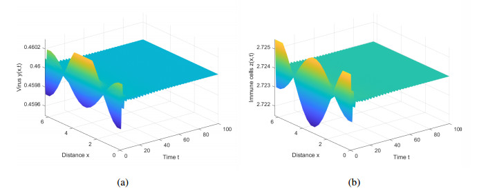
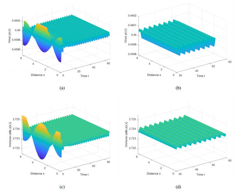
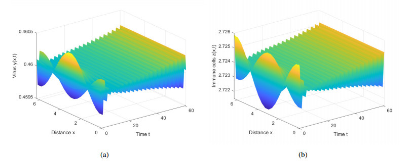
This paper introduces diffusion into an immunosuppressive infection model with virus stimulation delay and Beddington-DeAngelis functional response. First, we study the stability of positive constant steady state solution and show that the Hopf bifurcation will exist under certain conditions. Second, we derive the normal form of the Hopf bifurcation for the model reduced on the center manifold by using the multiple time scales (MTS) method. Moreover, the direction and stability of the bifurcating periodic solution are investigated. Finally, we present numerical simulations to verify the results of theoretical analysis and provide corresponding biological explanations.
- immunosuppressive infection model,
- Beddington-DeAngelis functional response,
- delay,
- Hopf bifurcation,
- multiple time scales
Citation: Yuan Xue, Jinli Xu, Yuting Ding. Dynamics analysis of a diffusional immunosuppressive infection model with Beddington-DeAngelis functional response[J]. Electronic Research Archive, 2023, 31(10): 6071-6088. doi: 10.3934/era.2023309

Related Papers:

Abstract

This paper introduces diffusion into an immunosuppressive infection model with virus stimulation delay and Beddington-DeAngelis functional response. First, we study the stability of positive constant steady state solution and show that the Hopf bifurcation will exist under certain conditions. Second, we derive the normal form of the Hopf bifurcation for the model reduced on the center manifold by using the multiple time scales (MTS) method. Moreover, the direction and stability of the bifurcating periodic solution are investigated. Finally, we present numerical simulations to verify the results of theoretical analysis and provide corresponding biological explanations.

References

[1]	N. L. Komarova, E. Barnes, P. Klenerman, D. Wodarz, Boosting immunity by antiviral drug therapy: a simple relationship among timing, efficacy, and success, Proc. Natl. Acad. Sci., 100 (2003), 1855–1860. https://doi.org/10.1073/pnas.0337483100 doi: 10.1073/pnas.0337483100
[2]	H. Dahari, A. Lo, R. M. Ribeiro, A. S. Perelson, Modeling hepatitis C virus dynamics: Liver regeneration and critical drug efficacy, J. Theor. Biol., 247 (2007), 371–381. https://doi.org/10.1016/j.jtbi.2007.03.006 doi: 10.1016/j.jtbi.2007.03.006
[3]	R. M. Anderson, G. F. Medley, R. M. May, A. M. Johnson, A preliminary study of the transmission dynamics of the human immunodeficiency virus (HIV), the causative agent of AIDS, Math. Med. Biol., 3 (1986), 229–263. https://doi.org/10.1093/imammb/3.4.229 doi: 10.1093/imammb/3.4.229
[4]	L. Zou, S. Ruan, W. Zhang, An age-structured model for the transmission dynamics of hepatitis B, SIAM J. Appl. Math., 70 (2010), 3121–3139. https://doi.org/10.1137/090777645 doi: 10.1137/090777645
[5]	R. S. Wijaya, S. A. Read, S. P. Selvamani, S. Schibeci, M. K. Azardaryany, A. Ong, et al., Hepatitis C virus (HCV) eradication with interferon-free direct-acting antiviral-based therapy results in KLRG1+ HCV-specific memory natural killer cells, J. Infect. Dis., 223 (2021), 1183–1195. https://doi.org/10.1093/infdis/jiaa492 doi: 10.1093/infdis/jiaa492
[6]	R. Wagner, J. T. Randolph, S. V. Patel, L. Nelson, M. A. Matulenko, R. Keddy, et al., Highlights of the structure-activity relationships of benzimidazole linked pyrrolidines leading to the discovery of the hepatitis C virus NS5A inhibitor pibrentasvir (ABT-530), J. Med. Chem., 61 (2018), 4052–4066. https://doi.org/10.1021/acs.jmedchem.8b00082 doi: 10.1021/acs.jmedchem.8b00082
[7]	A. Suk-Fong Lok, Hepatitis B treatment: what we know now and what remains to be researched, Hepatol. Commun., 3 (2019), 8–19. https://doi.org/10.1002/hep4.1281 doi: 10.1002/hep4.1281
[8]	Z. Meng, Y. Chen, M. Lu, Advances in targeting the innate and adaptive immune systems to cure chronic hepatitis B virus infection, Front. Immunol., 10 (2020), 3127. https://doi.org/10.3389/fimmu.2019.03127 doi: 10.3389/fimmu.2019.03127
[9]	M. P. Davenport, D. S. Khoury, D. Cromer, S. R. Lewin, A. D. Kelleher, S. J. Kent, Functional cure of HIV: the scale of the challenge, Nat. Rev. Immunol., 19 (2019), 45–54. https://doi.org/10.1038/s41577-018-0085-4 doi: 10.1038/s41577-018-0085-4
[10]	B. Autran, B. Descours, V. Avettand-Fenoel, C. Rouzioux, Elite controllers as a model of functional cure, Curr. Opin. HIV AIDS, 6 (2011), 181–187. https://doi.org/10.1097/COH.0b013e328345a328 doi: 10.1097/COH.0b013e328345a328
[11]	S. Shi, J. Huang, Y. Kuang, S. Ruan, Stability and Hopf bifurcation of a tumor-immune system interaction model with an immune checkpoint inhibitor, Commun. Nonlinear Sci. Numer. Simul., 118 (2023), 106996. https://doi.org/10.1016/j.cnsns.2022.106996 doi: 10.1016/j.cnsns.2022.106996
[12]	M. A. Benchaib, A. Bouchnita, V. Volpert, A. Makhoute, Mathematical modeling reveals that the administration of EGF can promote the elimination of lymph node metastases by PD-1/PD-L1 blockade, Front. Bioeng. Biotechnol., 7 (2019), 104. https://doi.org/10.3389/fbioe.2019.00104 doi: 10.3389/fbioe.2019.00104
[13]	A. Friedman, X. Lai, Combination therapy for cancer with oncolytic virus and checkpoint inhibitor: A mathematical model, PLoS One, 13 (2018), e0192449. https://doi.org/10.1371/journal.pone.0192449 doi: 10.1371/journal.pone.0192449
[14]	H. Shu, L. Wang, J. Watmough, Sustained and transient oscillations and chaos induced by delayed antiviral immune response in an immunosuppressive infection model, J. Math. Biol., 68 (2014), 477–503. https://doi.org/10.1007/s00285-012-0639-1 doi: 10.1007/s00285-012-0639-1
[15]	C. Tian, W. Gan, P. Zhu, Stability analysis in a diffusional immunosuppressive infection model with delayed antiviral immune response, Math. Methods Appl. Sci., 40 (2017), 4001–4013. https://doi.org/10.1002/mma.4279 doi: 10.1002/mma.4279
[16]	J. Li, X. Ma, J. Li, D. Zhang, Dynamics of a chronic virus infection model with viral stimulation delay, Appl. Math. Lett., 122 (2021), 107547. https://doi.org/10.1016/j.aml.2021.107547 doi: 10.1016/j.aml.2021.107547
[17]	D. Wodarz, Killer Cell Dynamics: Mathematical and Computational Approaches to Immunology, Springer, New York, 2007. https://doi.org/10.1007/978-0-387-68733-9-1
[18]	R. J. De Boer, A. S. Perelson, Towards a general function describing T cell proliferation, J. Theor. Biol., 175 (1995), 567–576. https://doi.org/10.1006/jtbi.1995.0165 doi: 10.1006/jtbi.1995.0165
[19]	R. J. De Boer, A. S. Perelson, Target cell limited and immune control models of HIV infection: a comparison, J. Theor. Biol., 190 (1998), 201–214. https://doi.org/10.1006/jtbi.1997.0548 doi: 10.1006/jtbi.1997.0548
[20]	J. R. Beddington, Mutual interference between parasites or predators and its effect on searching efficiency, J. Anim. Ecol., 44 (1975), 331–340. https://doi.org/10.2307/3866 doi: 10.2307/3866
[21]	D. L. DeAngelis, R. A. Goldstein, R. V. O'Neill, A model for tropic interaction, Ecology, 56 (1975), 881–892. https://doi.org/10.2307/1936298 doi: 10.2307/1936298
[22]	R. S. Cantrell, C. Cosner, On the dynamics of predator-prey models with the Beddington-DeAngelis functional response, J. Math. Anal. Appl., 257 (2001), 206–222. https://doi.org/10.1006/jmaa.2000.7343 doi: 10.1006/jmaa.2000.7343
[23]	W. Chen, M. Wang, Qualitative analysis of predator-prey models with Beddington-DeAngelis fun-ctional response and diffusion, Math. Comput. Model., 42 (2005), 31–44. https://doi.org/10.1016/j.mcm.2005.05.013 doi: 10.1016/j.mcm.2005.05.013
[24]	T. W. Hwang, Global analysis of the predator-prey system with Beddington-DeAngelis functional response, J. Math. Anal. Appl., 281 (2003), 395–401. https://doi.org/10.1016/S0022-247X(02)00395-5 doi: 10.1016/S0022-247X(02)00395-5
[25]	D. Wodarz, Ecological and evolutionary principles in immunology, Ecol. Lett., 9 (2006), 694–705. https://doi.org/10.1111/j.1461-0248.2006.00921.x doi: 10.1111/j.1461-0248.2006.00921.x
[26]	A. M. Elaiw, S. A. Azoz, Global properties of a class of HIV infection models with Beddington-DeAngelis functional response, Math. Methods Appl. Sci., 36 (2013), 383–394. https://doi.org/10.1002/mma.2596 doi: 10.1002/mma.2596
[27]	G. Huang, W. Ma, Y. Takeuchi, Global analysis for delay virus dynamics model with Beddington-DeAngelis functional response, Appl. Math. Lett., 24 (2011), 1199–1203. https://doi.org/10.1016/j.aml.2011.02.007 doi: 10.1016/j.aml.2011.02.007
[28]	X. Wang, Y. Tao, X. Song, A delayed HIV-1 infection model with Beddington-DeAngelis functional response, Nonlinear Dyn., 62 (2010), 67–72. https://doi.org/10.1007/s11071-010-9699-1 doi: 10.1007/s11071-010-9699-1
[29]	Y. Chen, L. Wang, Z. Liu, Y. Wang, Complex dynamics for an immunosuppressive infection model with virus stimulation delay and nonlinear immune expansion, Qual. Theory Dyn. Syst., 22 (2023), 118. https://doi.org/10.1007/s12346-023-00814-y doi: 10.1007/s12346-023-00814-y

Reader Comments

Your name:*

Email:*
© 2023 the Author(s), licensee AIMS Press. This is an open access article distributed under the terms of the Creative Commons Attribution License (http://creativecommons.org/licenses/by/4.0)