ODTC: An online darknet traffic classification model based on multimodal self-attention chaotic mapping features

Jiangtao Zhai; Haoxiang Sun; Chengcheng Xu; Wenqian Sun; Jiangtao Zhai; Haoxiang Sun; Chengcheng Xu; Wenqian Sun

doi:10.3934/era.2023259

Electronic Research Archive

2023, Volume 31, Issue 8: 5056-5082. doi: 10.3934/era.2023259

Previous Article Next Article

Research article Special Issues

ODTC: An online darknet traffic classification model based on multimodal self-attention chaotic mapping features

School of Electronics and Information Engineering, Nanjing University of Information Science and Technology, Nanjing 210044, China

Received: 31 May 2023 Revised: 11 July 2023 Accepted: 11 July 2023 Published: 14 July 2023

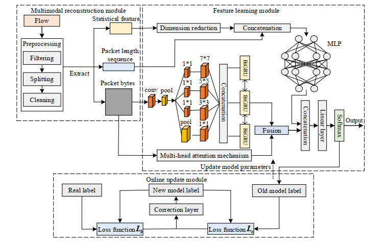
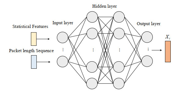
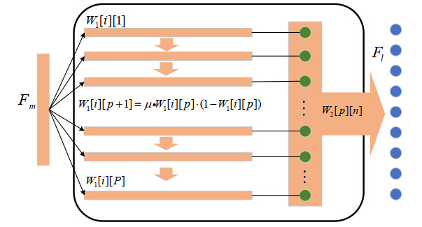
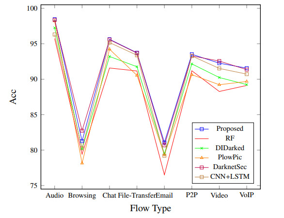
Darknet traffic classification is significantly important to network management and security. To achieve fast and accurate classification performance, this paper proposes an online classification model based on multimodal self-attention chaotic mapping features. On the one hand, the payload content of the packet is input into the network integrating CNN and BiGRU to extract local space-time features. On the other hand, the flow level abstract features processed by the MLP are introduced. To make up for the lack of the indistinct feature learning, a feature amplification module that uses logistic chaotic mapping to amplify fuzzy features is introduced. In addition, a multi-head attention mechanism is used to excavate the hidden relationships between different features. Besides, to better support new traffic classes, a class incremental learning model is developed with the weighted loss function to achieve continuous learning with reduced network parameters. The experimental results on the public CICDarketSec2020 dataset show that the accuracy of the proposed model is improved in multiple categories; however, the time and memory consumption is reduced by about 50$ % $. Compared with the existing state-of-the-art traffic classification models, the proposed model has better classification performance.
- darknet traffic,
- deep learning,
- logistic chaos map,
- multi-head self-attention mechanism,
- online parameter update
Citation: Jiangtao Zhai, Haoxiang Sun, Chengcheng Xu, Wenqian Sun. ODTC: An online darknet traffic classification model based on multimodal self-attention chaotic mapping features[J]. Electronic Research Archive, 2023, 31(8): 5056-5082. doi: 10.3934/era.2023259

Related Papers:

Abstract

Darknet traffic classification is significantly important to network management and security. To achieve fast and accurate classification performance, this paper proposes an online classification model based on multimodal self-attention chaotic mapping features. On the one hand, the payload content of the packet is input into the network integrating CNN and BiGRU to extract local space-time features. On the other hand, the flow level abstract features processed by the MLP are introduced. To make up for the lack of the indistinct feature learning, a feature amplification module that uses logistic chaotic mapping to amplify fuzzy features is introduced. In addition, a multi-head attention mechanism is used to excavate the hidden relationships between different features. Besides, to better support new traffic classes, a class incremental learning model is developed with the weighted loss function to achieve continuous learning with reduced network parameters. The experimental results on the public CICDarketSec2020 dataset show that the accuracy of the proposed model is improved in multiple categories; however, the time and memory consumption is reduced by about 50$ % $. Compared with the existing state-of-the-art traffic classification models, the proposed model has better classification performance.

References

[1]	A. Montieri, D. Ciuonzo, G. Bovenzi, V. Persico, A. Pescapé, A dive into the dark web: hierarchical traffic classification of anonymity tools, IEEE Trans. Network Sci. Eng., 7 (2019), 1043–1054. https://doi.org/10.1109/TNSE.2019.2901994 doi: 10.1109/TNSE.2019.2901994
[2]	G. Aceto, A. Pescapé, Internet censorship detection: a survey, Comput. Networks, 83 (2015), 381–421. https://doi.org/10.1016/j.comnet.2015.03.008 doi: 10.1016/j.comnet.2015.03.008
[3]	Y. D. Goli, R. Ambika, Network traffic classification techniques-a review, in 2018 International Conference on Computational Techniques, Electronics and Mechanical Systems (CTEMS), (2018), 219–222. https://doi.org/10.1109/CTEMS.2018.8769309
[4]	T. Bujlow, V. Carela-Español, P. Barlet-Ros Independent comparison of popular DPI tools for traffic classification, Comput. Networks, 76 (2015), 75–89. https://doi.org/10.1016/j.comnet.2014.11.001 doi: 10.1016/j.comnet.2014.11.001
[5]	S. Rezaei, X. Liu, Deep learning for encrypted traffic classification: an overview, IEEE Commun. Mag., 57 (2019), 76–81. https://doi.org/10.1109/MCOM.2019.1800819 doi: 10.1109/MCOM.2019.1800819
[6]	Y. Hu, F. Zou, L. Li, P. Yi, Traffic classification of user behaviors in Tor, I2P, ZeroNet, Freenet, in 2020 IEEE 19th International Conference on Trust, Security and Privacy in Computing and Communications (TrustCom), (2020), 418–424. https://doi.org/10.1109/TrustCom50675.2020.00064
[7]	Z. Fan, R. Liu, Investigation of machine learning based network traffic classification, in 2017 International Symposium on Wireless Communication Systems (ISWCS), (2017), 1–6. https://doi.org/10.1109/ISWCS.2017.8108090
[8]	N. Bayat, W. Jackson, D. Liu, Deep learning for network traffic classification, preprint, arXiv: 2106.12693.
[9]	X. Hu, C. Gu, F. Wei, CLD-Net: a network combining CNN and LSTM for internet encrypted traffic classification, Secur. Commun. Netw., 2021 (2021), 1–15. https://doi.org/10.1155/2021/5518460 doi: 10.1155/2021/5518460
[10]	A. H. Lashkari, G. Kaur, A. Rahali, Didarknet: a contemporary approach to detect and characterize the darknet traffic using deep image learning, in 2020 the 10th International Conference on Communication and Network Security, (2020), 1–13. https://doi.org/10.1145/3442520.3442521
[11]	K. Lin, X. Xu, H. Gao, TSCRNN: a novel classification scheme of encrypted traffic based on flow spatiotemporal features for efficient management of IIoT, Comput. Networks, 190 (2021), 107974. https://doi.org/10.1016/j.comnet.2021.107974 doi: 10.1016/j.comnet.2021.107974
[12]	K. Kim, J. H. Lee, H. K. Lim, S. W. Oh, Y. H. Han, Deep RNN-based network traffic classification scheme in edge computing system, Comput. Sci. Inf. Syst., 19 (2022), 165–184. https://doi.org/10.2298/CSIS200424038K doi: 10.2298/CSIS200424038K
[13]	J. Lan, X. Liu, B. Li, Y. Li, T. Geng, DarknetSec: a novel self-attentive deep learning method for darknet traffic classification and application identification, Comput. Secur., 116 (2022), 102663. https://doi.org/10.1016/j.cose.2022.102663 doi: 10.1016/j.cose.2022.102663
[14]	Z. Wu, Y. Dong, X. Qiu, J. Jin, Online multimedia traffic classification from the QoS perspective using deep learning, Comput. Networks, 204 (2022), 108716. https://doi.org/10.1016/j.comnet.2021.108716 doi: 10.1016/j.comnet.2021.108716
[15]	K. Shahbar, A. N. Zincir-Heywood, Effects of shared bandwidth on anonymity of the I2P network users, in 2017 IEEE Security and Privacy Workshops (SPW), (2017), 235–240. https://doi.org/10.1109/SPW.2017.19
[16]	Z. Rao, W. Niu, X. S. Zhang, H. Li, Tor anonymous traffic identification based on gravitational clustering, Peer-to-Peer Networking Appl., 11 (2018), 592–601. https://doi.org/10.1007/s12083-017-0566-4 doi: 10.1007/s12083-017-0566-4
[17]	L. A. Iliadis, T. Kaifas, Darknet traffic classification using machine learning techniques, in 2021 10th International Conference on Modern Circuits and Systems Technologies (MOCAST), (2021), 1–4. https://doi.org/10.1109/MOCAST52088.2021.9493386
[18]	M. B. Sarwar, M. K. Hanif, R. Talib, M. Younas, M. U. Sarwar, DarkDetect: darknet traffic detection and categorization using modified convolution-long short-term memory, IEEE Access, 9 (2021), 113705–113713. https://doi.org/10.1109/ACCESS.2021.3105000 doi: 10.1109/ACCESS.2021.3105000
[19]	T. Shapira, Y. Shavitt, FlowPic: a generic representation for encrypted traffic classification and applications identification, IEEE Trans. Netw. Serv. Manage., 18 (2021), 1218–1232. https://doi.org/10.1109/TNSM.2021.3071441 doi: 10.1109/TNSM.2021.3071441
[20]	H. Yao, C. Liu, P. Zhang, S. Wu, C. Jiang, S. Yu, Identification of encrypted traffic through attention mechanism based long short-term memory, IEEE Trans. Big Data, 8 (2022), 241–252. https://doi.org/10.1109/TBDATA.2019.2940675 doi: 10.1109/TBDATA.2019.2940675
[21]	J. Xie, S. Li, X. Yun, Y. Zhang, P. Chang, Hstf-model: an http-based trojan detection model via the hierarchical spatio-temporal features of traffics, Comput. Secur., 96 (2020), 101923. https://doi.org/10.1016/j.cose.2020.101923 doi: 10.1016/j.cose.2020.101923
[22]	M. M. Hassan, A. Gumaei, A. Alsanad, M. Alrubaian, G. Fortino, A hybrid deep learning model for efficient intrusion detection in big data environment, Inf. Sci., 513 (2020), 386–396. https://doi.org/10.1016/j.ins.2019.10.069 doi: 10.1016/j.ins.2019.10.069
[23]	P. R. Kanna, P. Santhi, Unified deep learning approach for efficient intrusion detection system using integrated spatial–temporal features, Knowledge-Based Syst., 226 (2021), 107132. https://doi.org/10.1016/j.knosys.2021.107132 doi: 10.1016/j.knosys.2021.107132
[24]	L. Liu, J. Zhen, G. Li, G. Zhan, Z. He, B. Du, et al., Dynamic spatial-temporal representation learning for traffic flow prediction, IEEE Trans. Intell. Transp. Syst., 22 (2021), 7169–7183. https://doi.org/10.1109/TITS.2020.3002718 doi: 10.1109/TITS.2020.3002718
[25]	G. D'Angelo, F. Palmieri, Network traffic classification using deep convolutional recurrent autoencoder neural networks for spatial–temporal features extraction, J. Network Comput. Appl., 173 (2021), 102890. https://doi.org/10.1016/j.jnca.2020.102890 doi: 10.1016/j.jnca.2020.102890
[26]	M. Lopez-Martin, B. Carro, A. Sanchez-Esguevillas, J. Lloret, Network traffic classifier with convolutional and recurrent neural networks for internet of things, IEEE Access, 5 (2017), 18042–18050. https://doi.org/10.1109/ACCESS.2017.2747560 doi: 10.1109/ACCESS.2017.2747560
[27]	F. Xiao, GEJS: a generalized evidential divergence measure for multisource information fusion, IEEE Trans. Syst. Man Cybern.: Syst., 53 (2023), 2246–2258. https://doi.org/10.1109/TSMC.2022.3211498 doi: 10.1109/TSMC.2022.3211498
[28]	L. Vu, C. T. Bui, Q. U. Nguyen, A deep learning based method for handling imbalanced problem in network traffic classification, in Proceedings of the 8th International Symposium on Information and Communication Technology, (2017), 333–339. https://doi.org/10.1145/3155133.3155175
[29]	W. Wang, M. Zhu, J. Wang, X. Zeng, Z. Yang, End-to-end encrypted traffic classification with one-dimensional convolution neural networks, in 2017 IEEE International Conference on Intelligence and Security Informatics (ISI), (2017), 43–48. https://doi.org/10.1109/ISI.2017.8004872
[30]	C. Liu, L. He, G. Xiong, Z. Cao, Z. Li, FS-Net: a flow sequence network for encrypted traffic classification, in IEEE INFOCOM 2019 - IEEE Conference on Computer Communications, (2019), 1171–1179. https://doi.org/10.1109/INFOCOM.2019.8737507
[31]	G. Aceto, D. Ciuonzo, A. Montieri, A. Pescapé, DISTILLER: encrypted traffic classification via multimodal multitask deep learning, J. Network Comput. Appl., 183–184 (2021), 102985. https://doi.org/10.1016/j.jnca.2021.102985 doi: 10.1016/j.jnca.2021.102985
[32]	G. Xie, Q. Li, Y. Jiang, Self-attentive deep learning method for online traffic classification and its interpretability, Comput. Networks, 196 (2021), 108267. https://doi.org/10.1016/j.comnet.2021.108267 doi: 10.1016/j.comnet.2021.108267
[33]	G. Bovenzi, L. Yang, A. Finamore, G. Aceto, D. Ciuonzo, A. Pescapè, et al., A first look at class incremental learning in deep learning mobile traffic classification, preprint, arXiv: 2107.04464.
[34]	F. Hu, S. Zhang, X. Lin, L. Wu, N. Liao, Y. Song, Network traffic classification model based on attention mechanism and spatiotemporal features, EURASIP J. Inf. Secur., 2023 (2023), 1–25. https://doi.org/10.1186/s13635-023-00141-4 doi: 10.1186/s13635-023-00141-4
[35]	Z. Wang, B. Ma, Y. Zeng, X. Lin, K. Shi, Z. Wang, Differential preserving in XGBoost model for encrypted traffic classification, in 2022 International Conference on Networking and Network Applications (NaNA), (2022), 220–225. https://doi.org/10.1109/NaNA56854.2022.00044
[36]	Q. Lyu, X. Lu, Effective media traffic classification using deep learning, in Proceedings of the 2019 3rd International Conference on Compute and Data Analysis, (2019), 139–146. https://doi.org/10.1145/3314545.3316278
[37]	C. Y. Lin, B. H. Chen, W. Y. Lan, An efficient approach for encrypted traffic classification using CNN and bidirectional GRU, in 2022 2nd International Conference on Consumer Electronics and Computer Engineering (ICCECE), (2022), 368–373. https://doi.org/10.1109/ICCECE54139.2022.9712708
[38]	A. Velichko, Neural network for low-memory IoT devices and MNIST image recognition using kernels based on logistic map, Electronics, 9 (2020), 1432. https://doi.org/10.3390/electronics9091432 doi: 10.3390/electronics9091432
[39]	V. Tong, H. A. Tran, S. Souihi, A. Mellouk, A novel QUIC traffic classifier based on convolutional neural networks, in 2018 IEEE Global Communications Conference (GLOBECOM), (2018), 1–6. https://doi.org/10.1109/GLOCOM.2018.8647128
[40]	Y. Guo, Z. Li, Z. Li, G. Xiong, M. Jiang, G. Gou, FLAGB: focal loss based adaptive gradient boosting for imbalanced traffic classification, in 2020 International Joint Conference on Neural Networks (IJCNN), (2020), 1–8. https://doi.org/10.1109/IJCNN48605.2020.9207336
[41]	Z. Bu, B. Zhou, P. Cheng, K. Zhang, Z. Ling, Encrypted network traffic classification using deep and parallel network-in-network models, IEEE Access, 8 (2020), 132950–132959. https://doi.org/10.1109/ACCESS.2020.3010637 doi: 10.1109/ACCESS.2020.3010637
[42]	L. A. Iliadis, T. Kaifas, Darknet traffic classification using machine learning techniques, in 2021 10th International Conference on Modern Circuits and Systems Technologies (MOCAST), (2021), 1–4. https://doi.org/10.1109/MOCAST52088.2021.9493386
[43]	G. Draper-Gil, A. H. Lashkari, M. S. I. Mamun, A. A. Ghorbani, Characterization of encrypted and vpn traffic using time-related, in Proceedings of the 2nd International Conference on Information Systems Security and Privacy (ICISSP), (2016), 407–414. https://doi.org/10.5220/0005740704070414
[44]	A. H. Lashkari, G. Draper-Gil, M. S. I. Mamun, A. A. Ghorbani, Characterization of tor traffic using time based features, in Proceedings of the 3rd International Conference on Information Systems Security and Privacy (ICISSP 2017), (2017), 253–262. https://doi.org/10.5220/0006105602530262
[45]	Q. A. Al-Haija, M. Krichen, W. A. Elhaija, Machine-learning-based darknet traffic detection system for IoT applications, Electronics, 11 (2022), 556. https://doi.org/10.3390/electronics11040556 doi: 10.3390/electronics11040556
[46]	N. Rust-Nguyen, M. Stamp, Darknet traffic classification and adversarial attacks, preprint, arXiv: 2206.06371.
[47]	R. Wang, Y. Zhao, A survey on anonymous communication systems traffic identification and classification, in 2021 3rd International Conference on Advanced Information Science and System (AISS 2021), 36 (2021), 1–5. https://doi.org/10.1145/3503047.3503087
[48]	N. Rust-Nguyen, M. Stamp, Darknet traffic classification and adversarial attacks, preprint, arXiv: 2206.06371.

Reader Comments

Your name:*

Email:*
© 2023 the Author(s), licensee AIMS Press. This is an open access article distributed under the terms of the Creative Commons Attribution License (http://creativecommons.org/licenses/by/4.0)