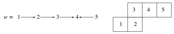
Recently, Çanakçi and Schroll proved that associated with a string module $ M(w) $ there is an appropriated snake graph $ \mathscr{G} $. They established a bijection between the corresponding perfect matching lattice $ \mathscr{L}(\mathscr{G}) $ of $ \mathscr{G} $ and the canonical submodule lattice $ \mathscr{L}(M(w)) $ of $ M(w) $. We introduce Brauer configurations whose polygons are defined by snake graphs in line with these results. The developed techniques allow defining snake graphs, which after suitable procedures, build Kronecker modules. We compute the dimension of the Brauer configuration algebras and their centers arising from the different processes. As an application, we estimate the trace norm of the canonical non-regular Kronecker modules and some families of trees associated with some snake graphs classes.
Citation: Agustín Moreno Cañadas, Pedro Fernando Fernández Espinosa, Natalia Agudelo Muñetón. Brauer configuration algebras defined by snake graphs and Kronecker modules[J]. Electronic Research Archive, 2022, 30(8): 3087-3110. doi: 10.3934/era.2022157
Recently, Çanakçi and Schroll proved that associated with a string module $ M(w) $ there is an appropriated snake graph $ \mathscr{G} $. They established a bijection between the corresponding perfect matching lattice $ \mathscr{L}(\mathscr{G}) $ of $ \mathscr{G} $ and the canonical submodule lattice $ \mathscr{L}(M(w)) $ of $ M(w) $. We introduce Brauer configurations whose polygons are defined by snake graphs in line with these results. The developed techniques allow defining snake graphs, which after suitable procedures, build Kronecker modules. We compute the dimension of the Brauer configuration algebras and their centers arising from the different processes. As an application, we estimate the trace norm of the canonical non-regular Kronecker modules and some families of trees associated with some snake graphs classes.

| [1] |
A. M. Cañadas, I. D. M. Gaviria, J. D. C. Vega, Relationships between the Chicken McNugget problem, Mutations of Brauer configuration algebras and the advanced encryption standard, Mathematics, 9 (2021), 1937. https://doi.org/10.3390/math9161937 doi: 10.3390/math9161937

|
| [2] |
A. M. Cañadas, M. A. O. Angarita, Brauer configuration algebras for multimedia based cryptography and security applications, Multimed. Tools Appl., 80 (2021), 23485–23510. https://doi.org/10.1007/s11042-020-10239-3 doi: 10.1007/s11042-020-10239-3
|
| [3] |
N. Agudelo, A. M. Cañadas, I. D. M. Gaviria, P. F. F. Espinosa, $\{0, 1\}$-Brauer configuration algebras and their applications in the graph energy theory, Mathematics, 9 (2021), 3042. https://doi.org/10.3390/math9233042 doi: 10.3390/math9233042
|
| [4] |
E. L. Green, S. Schroll, Brauer configuration algebras: A generalization of Brauer graph algebras, Bull. Sci. Math., 121 (2017), 539–572. https://doi.org/10.1016/j.bulsci.2017.06.001 doi: 10.1016/j.bulsci.2017.06.001
|
| [5] | S. Schroll, Brauer graph algebras, in Homological Methods, Representation Theory, and Cluster Algebras, Springer, (2018), 177–223. https://doi.org/10.1007/978-3-319-74585-5 |
| [6] |
J. Propp, The combinatorics of frieze patterns and Markoff numbers, Integers, 20 (2020), 1–38. https://doi.org/10.48550/arXiv.math/0511633 doi: 10.48550/arXiv.math/0511633
|
| [7] |
I. Çanakçi, R. Schiffler, Cluster algebras and continued fractions, Compos. Math., 54 (2018), 565–593. https://doi.org/10.1112/S0010437X17007631 doi: 10.1112/S0010437X17007631
|
| [8] |
I. Çanakçi, R. Schiffler, Snake graphs and continued fractions, Eur. J. Combin., 86 (2020), 1–19. https://doi.org/10.1016/j.ejc.2020.103081 doi: 10.1016/j.ejc.2020.103081
|
| [9] |
I. Çanakçi, R. Schiffler, Snake graphs calculus and cluster algebras from surfaces, J. Algebra, 382 (2013), 240–281. https://doi.org/10.1016/j.jalgebra.2013.02.018 doi: 10.1016/j.jalgebra.2013.02.018
|
| [10] |
I. Çanakçi, R. Schiffler, Snake graphs calculus and cluster algebras from surfaces Ⅱ: Self-crossings snake graphs, Math. Z., 281 (2015), 55–102. https://doi.org/10.1007/s00209-015-1475-y doi: 10.1007/s00209-015-1475-y
|
| [11] | I. Çanakçi, R. Schiffler, Snake graphs calculus and cluster algebras from surfaces Ⅲ: Band graphs and snake rings, Int. Math. Res. Not. IMRN, (2019), 1145–1226. |
| [12] |
I. Çanakçi, S. Schroll, Lattice bijections for string modules snake graphs and the weak Bruhat order, Adv. Appl. Math., 126, (2021), 102094. https://doi.org/10.1016/j.aam.2020.102094 doi: 10.1016/j.aam.2020.102094
|
| [13] | G. E. Andrews, The Theory of Partitions, Cambridge University Press, Cambridge UK, 2010. |
| [14] |
A. Sierra, The dimension of the center of a Brauer configuration algebra. J. Algebra, 510 (2018), 289–318. https://doi.org/10.1016/j.jalgebra.2018.06.002 doi: 10.1016/j.jalgebra.2018.06.002
|
| [15] | P. F. F. Espinosa, Categorification of some integer sequences and its applications, Ph.D thesis, Universidad Nacional de Colombia, BTA, Colombia, 2021. |
| [16] | D. Simson, Linear Representations of Partially Ordered Sets and Vector Space Categories, Gordon and Breach, London UK, 1992. |
| [17] |
A. M. Cañadas, I. D. M. Gaviria, P. F. F. Espinosa, Brauer configuration algebras and Kronecker modules to categorify integer sequences, ERA, 30 (2022), 661–682. https://doi.org/10.3934/era.2022035 doi: 10.3934/era.2022035
|
Figures(17)
Agustín Moreno Cañadas, Pedro Fernando Fernández Espinosa, Natalia Agudelo Muñetón. Brauer configuration algebras defined by snake graphs and Kronecker modules[J]. Electronic Research Archive, 2022, 30(8): 3087-3110. doi: 10.3934/era.2022157


 DownLoad: