Control analysis of optogenetics and deep brain stimulation targeting basal ganglia for Parkinson's disease

Honghui Zhang; Yuzhi Zhao; Zhuan Shen; Fangyue Chen; Zilu Cao; Wenxuan Shan; Honghui Zhang; Yuzhi Zhao; Zhuan Shen; Fangyue Chen; Zilu Cao; Wenxuan Shan

doi:10.3934/era.2022115

Electronic Research Archive

2022, Volume 30, Issue 6: 2263-2282. doi: 10.3934/era.2022115

Previous Article Next Article

Research article Special Issues

Control analysis of optogenetics and deep brain stimulation targeting basal ganglia for Parkinson's disease

1.
School of Mathematics and Statistics, Northwestern Polytechnical University, 1 Dongxiang Road, Chang'an District, Xi'an, Shaanxi, 710129, China
2.
MIIT Key Laboratory of Dynamics and Control of Complex Systems, 1 Dongxiang Road, Chang'an District, Xi'an, Shaanxi, 710129, China

Received: 29 September 2021 Revised: 18 December 2021 Accepted: 20 December 2021 Published: 21 April 2022

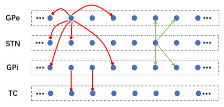
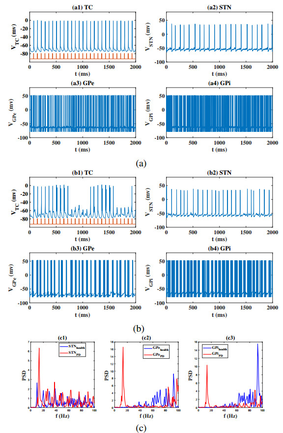
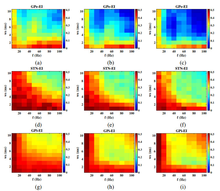
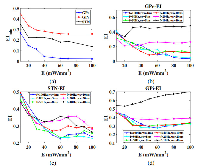
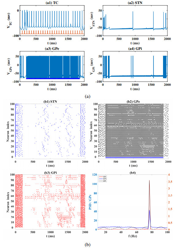
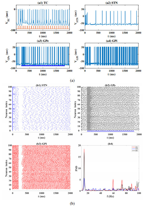
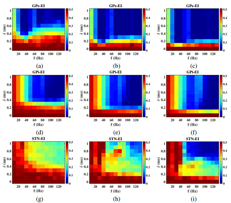
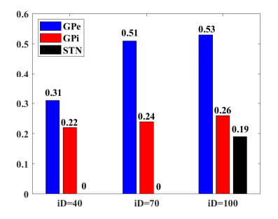
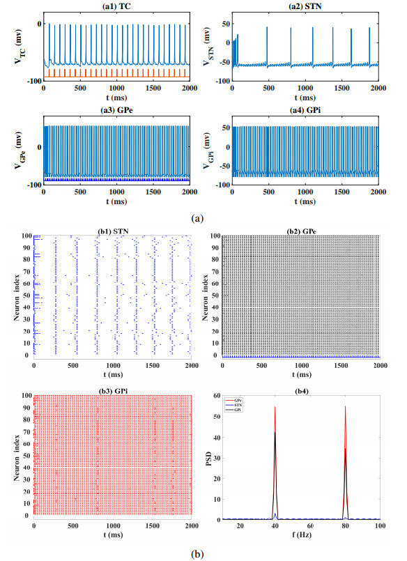
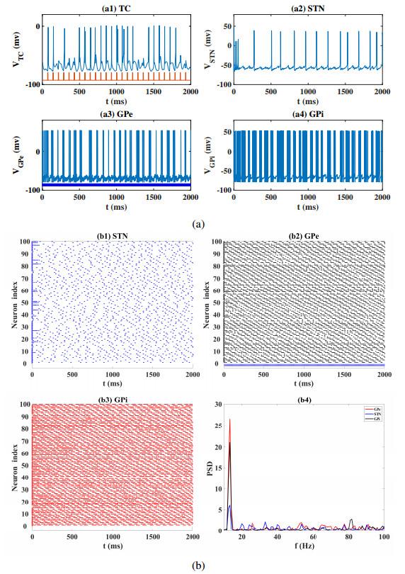
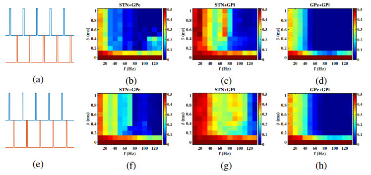
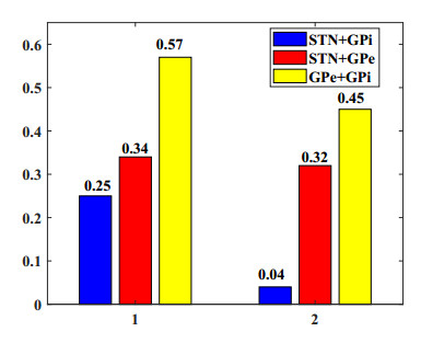
Interested in the regulatory effects of emerging optogenetics and classical deep brain stimulation (DBS) on Parkinson's disease (PD), through analysis of thalamic fidelity, here we conduct systematic work with the help of biophysically-based basal ganglia-thalamic circuits model. Under the excitatory ChannelRhodopsin-2 (ChR2), results show that photostimulation targeting globus pallidus externa (GPe) can restore the thalamic relay ability, reduce the synchrony of neurons and alleviate the excessive beta band oscillation, while the effects of targeting globus pallidus interna (GPi) and subthalamic nucleus (STN) are poor. To our delight, these results match experimental reports that the symptoms of PD's movement disorder can be alleviated effectively when GPe are excited by optogenetic, but the situation for STN is not satisfactory. For DBS, we also get considerable simulation results after stimulating GPi, STN and GPe. And the control effect of targeting GPe is better than that of GPi as revealed in some experiments. Furthermore, to reduce side effects and electrical energy, six different dual target combination stimulation strategies are compared, among which the combination of GPe and GPi is the best. Most noteworthy, GPe is shown to be a potential target for both electrical and photostimulation. Although these results need further clinical and experimental verification, they are still expected to provide some enlightenment for the treatment of PD.
- basal ganglia-thalamic network,
- optogenetics,
- deep brain stimulation (DBS),
- Parkinson's disease (PD),
- thalamic fidelity
Citation: Honghui Zhang, Yuzhi Zhao, Zhuan Shen, Fangyue Chen, Zilu Cao, Wenxuan Shan. Control analysis of optogenetics and deep brain stimulation targeting basal ganglia for Parkinson's disease[J]. Electronic Research Archive, 2022, 30(6): 2263-2282. doi: 10.3934/era.2022115

Related Papers:

Abstract

Interested in the regulatory effects of emerging optogenetics and classical deep brain stimulation (DBS) on Parkinson's disease (PD), through analysis of thalamic fidelity, here we conduct systematic work with the help of biophysically-based basal ganglia-thalamic circuits model. Under the excitatory ChannelRhodopsin-2 (ChR2), results show that photostimulation targeting globus pallidus externa (GPe) can restore the thalamic relay ability, reduce the synchrony of neurons and alleviate the excessive beta band oscillation, while the effects of targeting globus pallidus interna (GPi) and subthalamic nucleus (STN) are poor. To our delight, these results match experimental reports that the symptoms of PD's movement disorder can be alleviated effectively when GPe are excited by optogenetic, but the situation for STN is not satisfactory. For DBS, we also get considerable simulation results after stimulating GPi, STN and GPe. And the control effect of targeting GPe is better than that of GPi as revealed in some experiments. Furthermore, to reduce side effects and electrical energy, six different dual target combination stimulation strategies are compared, among which the combination of GPe and GPi is the best. Most noteworthy, GPe is shown to be a potential target for both electrical and photostimulation. Although these results need further clinical and experimental verification, they are still expected to provide some enlightenment for the treatment of PD.

References

[1]	I. Banegas, I. Prieto, A. Segarra, M. de Gasparo, M. Ramírez-Sánchez, Study of the neuropeptide function in Parkinson's disease using the 6-Hydroxydopamine model of experimental Hemiparkinsonism, AIMS Neurosci., 4 (2017), 223–237. https://doi.org/10.3934/Neuroscience.2017.4.223 doi: 10.3934/Neuroscience.2017.4.223
[2]	A. Galvan, T. Wichmann, Pathophysiology of parkinsonism, Clin. Neurophysiol., 119 (2008), 1459–1474. https://doi.org/10.1016/j.clinph.2008.03.017 doi: 10.1016/j.clinph.2008.03.017
[3]	H. Zhang, Y. Yu, Z. Deng, Q. Wang, Activity pattern analysis of the subthalamopallidal network under ChannelRhodopsin-2 and Halorhodopsin photocurrent control, Chaos Solitons Fractals, 138 (2020), 109963. https://doi.org/10.1016/j.chaos.2020.109963 doi: 10.1016/j.chaos.2020.109963
[4]	Y. Yu, X. Wang, Q. Wang, Q. Wang, A review of computational modeling and deep brain stimulation: applications to Parkinson's disease, Appl. Math. Mech., 41 (2020), 1747–1768. https://doi.org/10.1007/s10483-020-2689-9 doi: 10.1007/s10483-020-2689-9
[5]	J. E. Rubin, D. Terman, High frequency stimulation of the subthalamic nucleus eliminates pathological thalamic rhythmicity in a computational model, J. Comput. Neurosci., 16 (2004), 211–235. https://doi.org/10.1023/B:JCNS.0000025686.47117.67 doi: 10.1023/B:JCNS.0000025686.47117.67
[6]	R. Q. So, A. R. Kent, W. M. Grill, Relative contributions of local cell and passing fiber activation and silencing to changes in thalamic fidelity during deep brain stimulation and lesioning: a computational modeling study, J. Comput. Neurosci., 32 (2012), 499–519. https://doi.org/10.1007/s10827-011-0366-4 doi: 10.1007/s10827-011-0366-4
[7]	K. Kumaravelu, D. T. Brocker, W. M. Grill, A biophysical model of the cortex-basal ganglia-thalamus network in the 6-OHDA lesioned rat model of Parkinson's disease, J. Comput. Neurosci., 40 (2016), 207–229.
[8]	Y. Yu, Y. Hao, Q. Wang, Model-based optimized phase-deviation deep brain stimulation for Parkinson's disease, Neural Netw., 122 (2020), 308–319. https://doi.org/10.1016/j.neunet.2019.11.001 doi: 10.1016/j.neunet.2019.11.001
[9]	C. Yu, I. R. Cassar, J. Sambangi, W. M. Grill, Frequency-specific optogenetic deep brain stimulation of subthalamic nucleus improves parkinsonian motor behaviors, J. Neurosci., 40 (2020), 4323–4334. https://doi.org/10.1523/JNEUROSCI.3071-19.2020 doi: 10.1523/JNEUROSCI.3071-19.2020
[10]	K. J. Mastro, K. T. Zitelli, A. M. Willard, K. H. Leblanc, A. V. Kravitz, A. H. Gittis, Cell-specific pallidal intervention induces long-lasting motor recovery in dopamine-depleted mice, Nature Neurosci., 20 (2017), 815–823. https://doi.org/10.1038/nn.4559 doi: 10.1038/nn.4559
[11]	S. Ratnadurai-Giridharan, C. C. Cheung, L. L. Rubchinsky, Effects of electrical and optogenetic deep brain stimulation on synchronized oscillatory activity in parkinsonian basal ganglia, IEEE Trans. Neural Syst. Rehabilitation Eng., 25 (2017), 2188–2195. https://doi.org/10.1109/TNSRE.2017.2712418 doi: 10.1109/TNSRE.2017.2712418
[12]	Y. Yu, F. Han, Q. Wang, Q. Wang, Model-based optogenetic stimulation to regulate beta oscillations in Parkinsonian neural networks, Cogn. Neurodyn., (2021), 1–15. https://doi.org/10.1007/s11571-021-09729-3 doi: 10.1007/s11571-021-09729-3
[13]	T. Ishizuka, M. Kakuda, R. Araki, H. Yawo, Kinetic evaluation of photosensitivity in genetically engineered neurons expressing green algae light-gated channels, Neurosci. Res., 54 (2006), 85–94. https://doi.org/10.1016/j.neures.2005.10.009 doi: 10.1016/j.neures.2005.10.009
[14]	K. Nikolic, P. Degenaar, C. Toumazou, Modeling and Engineering aspects of ChannelRhodopsin2 System for Neural Photostimulation, Conf. Proc. IEEE Eng. Med. Biol. Soc., (2006), 1626–1629. https://doi.org/10.1109/IEMBS.2006.260766 doi: 10.1109/IEMBS.2006.260766
[15]	R. A. Stefanescu, R. G. Shivakeshavan, P. P. Khargonekar, S. S. Talathi, Computational modeling of channelrhodopsin-2 photocurrent characteristics in relation to neural signaling, Bull. Math. Biol., 75 (2013), 2208–2240. https://doi.org/10.1007/s11538-013-9888-4 doi: 10.1007/s11538-013-9888-4
[16]	P. Krack, A. Batir, N. V. Blercom, S. Chabardes, P. Pollak, Five-year follow-up of bilateral stimulation of the subthalamic nucleus in advanced Parkinson's disease, N. Engl. J. Med., 349 (2003), 1925–1934. https://doi.org/10.1056/NEJMoa035275 doi: 10.1056/NEJMoa035275
[17]	U. Knoblich, F. Zhang, K. Deisseroth, L. H. Tsai, C. I. Moore, J. A. Cardin, et al., Targeted optogenetic stimulation and recording of neurons in vivo using cell-type-specific expression of Channelrhodopsin-2, Nat. Protoc., 5 (2010), 247–254.
[18]	V. Gradinaru, M. Mogri, K. R. Thompson, J. M. Henderson, K. Deisseroth, Optical deconstruction of parkinsonian neural circuitry, Science, 324 (2009), 354–359. https://doi.org/10.1126/science.1167093 doi: 10.1126/science.1167093
[19]	H. H. Yoon, M.-H. Nam, I. Choi, J. Min, S. R. Jeon, Optogenetic inactivation of the entopeduncular nucleus improves forelimb akinesia in a parkinson's disease model, Behav. Brain Res., 386 (2020), 112551. https://doi.org/10.1016/j.bbr.2020.112551 doi: 10.1016/j.bbr.2020.112551
[20]	M. Daneshzand, S. A. Ibrahim, M. Faezipour, B. D. Barkana, Desynchronization and energy efficiency of gaussian neurostimulation on different sites of the basal ganglia, in IEEE Int. Conf. Bio-Informatics and Bio-Eng. (IEEE BIBE), (2017), 57–62. https://doi.org/10.1109/BIBE.2017.00-78

Reader Comments

Your name:*

Email:*
© 2022 the Author(s), licensee AIMS Press. This is an open access article distributed under the terms of the Creative Commons Attribution License (http://creativecommons.org/licenses/by/4.0)