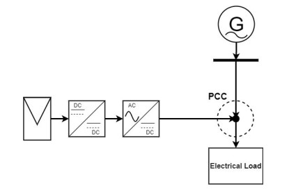
Residential photovoltaic systems are a cost-effective solution for Palestinians to reduce their power costs while improving the environment. Despite their numerous advantages, these systems have several negative effects on the entire electric grid infrastructure. Increased penetration of photovoltaic (PV) systems, for example, may result in a fall in the power factor of the distribution grid. When the power factor is low, heat production and switch failures are more likely to occur. Even though comparable research has been published in the past, this is the first time PV systems have been investigated in terms of power factors in Palestine. This research serves as a resource for people interested in how photovoltaics (PVs) impact their systems' total power factor. To begin, the researchers in this study presented an intuitive power factor selection criterion for photovoltaic (PV) systems. Second, the article included a proposal for an auxiliary power factor controller. This article's conclusions may be utilized by municipalities, grid operators, and legislators to aid them in planning, forecasting, and accommodating new PV systems in their grids in terms of total power factor, as demonstrated by the results of this study. However, even though the data in this study is drawn from Palestinian sources, it may be applied to other regions because the data sets used are worldwide in scope.
Citation: Amer Braik, Asaad Makhalfih, Ag Sufiyan Abd Hamid, Kamaruzzaman Sopian, Adnan Ibrahim. Impact of photovoltaic grid-tied systems on national grid power factor in Palestine[J]. AIMS Energy, 2022, 10(2): 236-253. doi: 10.3934/energy.2022013
Residential photovoltaic systems are a cost-effective solution for Palestinians to reduce their power costs while improving the environment. Despite their numerous advantages, these systems have several negative effects on the entire electric grid infrastructure. Increased penetration of photovoltaic (PV) systems, for example, may result in a fall in the power factor of the distribution grid. When the power factor is low, heat production and switch failures are more likely to occur. Even though comparable research has been published in the past, this is the first time PV systems have been investigated in terms of power factors in Palestine. This research serves as a resource for people interested in how photovoltaics (PVs) impact their systems' total power factor. To begin, the researchers in this study presented an intuitive power factor selection criterion for photovoltaic (PV) systems. Second, the article included a proposal for an auxiliary power factor controller. This article's conclusions may be utilized by municipalities, grid operators, and legislators to aid them in planning, forecasting, and accommodating new PV systems in their grids in terms of total power factor, as demonstrated by the results of this study. However, even though the data in this study is drawn from Palestinian sources, it may be applied to other regions because the data sets used are worldwide in scope.

| [1] | PCBS (2021, May 26). Estimated Population in the Palestine Mid-Year by Governorate, 1997-2026. Palestinian Central Bureau of Statistics. Retrieved November 19, 2021, Available from: https://www.pcbs.gov.ps/statisticsIndicatorsTables.aspx?lang=en&table_id=676. |
| [2] | (PENRA), P.E.a.N.R.A. Paving the Way for a Renewable Energy Future in Palestine. Available from: http://www.penra.pna.ps/ar/Uploads/Files/Electric%20power%20in%20Palestine%202016-2019.pdf. |
| [3] |
Khatib T, Bazyan A, Assi H, et al. (2021) Palestine energy policy for photovoltaic generation: Current status and what should be next? Sustainability 13: 2996. https://doi.org/10.3390/su13052996 doi: 10.3390/su13052996

|
| [4] | Sukarno K, Hamid ASA, Razali H, et al. (2017) Evaluation on cooling effect on solar PV power output using Laminar H2O surface method. Int J Renewable Energy Res 7: 1213-1218. |
| [5] |
Ahmad EZ, Sopian K, Jarimi H, et al. (2021) Recent advances in passive cooling methods for photovoltaic performance enhancement. Int J Electr Comput Eng 11: 146. https://doi.org/10.11591/ijece.v11i1.pp146-154 doi: 10.11591/ijece.v11i1.pp146-154
|
| [6] |
Ueda Y, Kurokawa K, Kitamura K, et al. (2009) Performance analysis of various system configurations on grid-connected residential PV systems. Sol Energy Mater Sol Cells 93: 945-949. https://doi.org/10.1016/j.solmat.2008.11.021 doi: 10.1016/j.solmat.2008.11.021
|
| [7] |
Monna S, Juaidi A, Abdallah R, et al. (2020) A comparative assessment for the potential energy production from PV installation on residential buildings. Sustainability 12: 10344. https://doi.org/10.3390/su122410344 doi: 10.3390/su122410344
|
| [8] |
Sugiura T, Yamada T, Nakamura H, et al. (2003) Measurements, analyses and evaluation of residential PV systems by Japanese monitoring program. Sol Energy Mater Sol Cells 75: 767-779. https://doi.org/10.1016/S0927-0248(02)00132-0 doi: 10.1016/S0927-0248(02)00132-0
|
| [9] | Baran ME, Hooshyar H, Shen Z, et al. (2011) Impact of high penetration residential PV systems on distribution systems. In Proceedings of the 2011 IEEE Power and Energy Society General Meeting, IEEE, 1-5. https://doi.org/10.1109/PES.2011.6039799 |
| [10] |
Leloux J, Narvarte L, Trebosc D (2012) Review of the performance of residential PV systems in France. Renewable Sustainable Energy Rev 16: 1369-1376. https://doi.org/10.1016/j.rser.2011.10.018 doi: 10.1016/j.rser.2011.10.018
|
| [11] |
Omar MA, Mahmoud MM (2018) Grid connected PV-home systems in Palestine: A review on technical performance, effects and economic feasibility. Renewable Sustainable Energy Rev 82: 2490-2497. https://doi.org/10.1016/j.rser.2017.09.008 doi: 10.1016/j.rser.2017.09.008
|
| [12] |
Weniger J, Tjaden T, Quaschning V (2014) Sizing of residential PV battery systems. Energy Procedia 46: 78-87. https://doi.org/10.1016/j.egypro.2014.01.160 doi: 10.1016/j.egypro.2014.01.160
|
| [13] |
Watts D, Valdés MF, Jara D, et al. (2015) Potential residential PV development in Chile: The effect of Net Metering and Net Billing schemes for grid-connected PV systems. Renewable Sustainable Energy Rev 41: 1037-1051. https://doi.org/10.1016/j.rser.2014.07.201 doi: 10.1016/j.rser.2014.07.201
|
| [14] |
Amuzuvi CK (2014) Design of a photovoltaic system as an alternative source of electrical energy for powering the lighting circuits for premises in Ghana. J Electr Electron Eng 2: 9. https://doi.org/10.11648/j.jeee.20140201.12 doi: 10.11648/j.jeee.20140201.12
|
| [15] |
Camilo FM, Castro R, Almeida ME, et al. (2017) Economic assessment of residential PV systems with self-consumption and storage in Portugal. Sol Energy 150: 353-362. https://doi.org/10.1016/j.solener.2017.04.062 doi: 10.1016/j.solener.2017.04.062
|
| [16] | Guo L, Cheng Y, Zhang L, et al. (2008) Research on power—factor regulating tariff standard. International Conference on Electricity Distribution. In Proceedings of the IEEE, China. |
| [17] |
Kawasaki S, Kanemoto N, Taoka H, et al. (2012) Cooperative voltagecontrol method by power factor control of PV systems and LRT. IEEJ Trans Power Energy 132: 309-316. https://doi.org/10.1541/ieejpes.132.309 doi: 10.1541/ieejpes.132.309
|
| [18] |
Malengret M, Gaunt CT (2020) Active currents, power factor, and apparent power for practical power delivery systems. IEEE Access 8: 133095-133113. https://doi.org/10.1109/ACCESS.2020.3010638 doi: 10.1109/ACCESS.2020.3010638
|
| [19] |
Emmanuel M, Rayudu R, Welch I (2017) Impacts of power factor control schemes in time series power flow analysis for centralized PV plants using Wavelet Variability Model. IEEE Trans Ind Informatics 13: 3185-3194. https://doi.org/10.1109/TⅡ.2017.2702183 doi: 10.1109/TⅡ.2017.2702183
|
| [20] | Peng W, Baghzouz Y, Haddad S (2013) Local load power factor correction by grid-interactive PV inverters. In Proceedings of the 2013 IEEE Grenoble Conference; IEEE, 1-6. https://doi.org/10.1109/PTC.2013.6652412 |
| [21] |
Gusman LS, Pereira HA, Callegari JMS, et al. (2020) Design for reliability of multifunctional PV inverters used in industrial power factor regulation. Int J Electr Power Energy Syst 119: 105932. https://doi.org/10.1016/j.ijepes.2020.105932 doi: 10.1016/j.ijepes.2020.105932
|
| [22] |
Hassaine L, Olias E, Quintero J, et al. (2009) Digital power factor control and reactive power regulation for grid-connected photovoltaic inverter. Renewable Energy 34: 315-321. https://doi.org/10.1016/j.renene.2008.03.016 doi: 10.1016/j.renene.2008.03.016
|
| [23] |
Rani PS (2020) Enhancement of power quality in grid connected PV system. Indian J Sci Technol 13: 3630-3641. https://doi.org/10.17485/IJST/v13i35.1266 doi: 10.17485/IJST/v13i35.1266
|
| [24] | Aziz A, Purwar V (2017) Simulation of high power factor single phase inverter for PV solar array : A survey. 0869: 174-177. |
| [25] | Solutions, GSE, Power Factor and Grid-Connected Photovoltaics. 2015. Available from: https://www.gses.com.au/wp-content/uploads/2016/03/GSES_powerfactor-110316.pdf. |
| [26] | Electric S. How to avoid power factor degradation due to the integration of solar production? Available from: https://www.electrical-installation.org/enwiki/Power_factor_-_impact_of_solar_self-consumption. |
| [27] | Power L. Understanding the effects of introducing solar PV and how it can affect "Power Factor" on complex Industrial/Commercial sites; Available from: https://www.livingpower.com.au/power-factor. |
| [28] | NEDCO. PV Net Metering System Instructions. Available from: http://www.nedco.ps/?ID=1536. |
| [29] | JDECO. PV Plants Building Instructions. Available from: https://www.jdeco.net/ar_folder.aspx?id=FWg0CFa23793825aFWg0CF. |
| [30] | Magazine P (2019) Palestine to bring online its first PV plant, at 7.5 MW. Available from: https://www.pv-magazine.com/2019/05/24/palestine-to-bring-online-its-first-pv-plant-at-7-5-mw/. |
| [31] | Authority, P.E.a.N.R. Energy Policy Articles 2020; Available from: http://www.penra.pna.ps/ar/index.php?p=penra6. |
| [32] | Bullich-massagu E, Ferrer-san-jos R, Serrano-salamanca L, Pacheco-navas, C.; Gomis-bellmunt, O. PowerPlantControl. Available from: http://dx.doi.org/10.1049/iet-rpg.2015.0113. |
| [33] | Bernáth F, Mastný P. Power Factor Compensation of Photovoltaic Power Plant. 2012, 0-4. Available from: https://core.ac.uk/download/pdf/295548557.pdf. |
| [34] | University, B. Birzeit University and Qudra inaugurate a 1 megawatt solar power plant. 2021; Available from: https://www.birzeit.edu/en/node/45562. |
| [35] | Solutions, Q.f.R.E. Qudra for Renewable Energy Solutions begins operating a 1 megawatt solar power plant for the Yabad Electricity Authority. 2021. Available from: https://www.wattan.net/ar/news/336254.html. |
| [36] | Daud MZ, Mohamed A, Che Wanik MZ, et al. (2012) Performance evaluation of Grid-Connected photovoltaic system with battery energy storage. IEEE International Conference on Power and Energy (PECon). https://doi.org/10.1109/PECon.2012.6450234 |
| [37] |
Assadeg J, Sopian K, Fudholi A (2019) Performance of grid-connected solar photovoltaic power plants in the Middle East and North Africa. Int J Electr Comput Eng (IJECE) 9: 3375. https://doi.org/10.11591/ijece.v9i5.pp3375-3383 doi: 10.11591/ijece.v9i5.pp3375-3383
|
| [38] |
Farhoodnea M, Mohamed A, Khatib T, et al. (2015) Performance evaluation and characterization of a 3-kWp grid-connected photovoltaic system based on tropical field experimental results: new results and comparative study. Renewable Sustainable Energy Rev 42: 1047-1054. https://doi.org/10.1016/j.rser.2014.10.090 doi: 10.1016/j.rser.2014.10.090
|
| [39] |
Kamaruzzaman Z, Mohamed A, Shareef H (2015) Effect of grid-connected photovoltaic systems on static and dynamic voltage stability with analysis techniques—a review. PRZEGLĄD ELEKTROTECHNICZNY 1: 136-140. https://doi.org/10.15199/48.2015.06.27 doi: 10.15199/48.2015.06.27
|
| [40] | Farhoodnea M, Mohamed A, Shareef H, et al. (2013) Power quality analysis of Grid-Connected photovoltaic systems in distribution networks. PRZEGLĄD ELEKTROTECHNICZNY. https://doi.org/10.1109/SCOReD.2012.6518600 |


Figures(13) / Tables(3)

Amer Braik, Asaad Makhalfih, Ag Sufiyan Abd Hamid, Kamaruzzaman Sopian, Adnan Ibrahim. Impact of photovoltaic grid-tied systems on national grid power factor in Palestine[J]. AIMS Energy, 2022, 10(2): 236-253. doi: 10.3934/energy.2022013


 DownLoad: