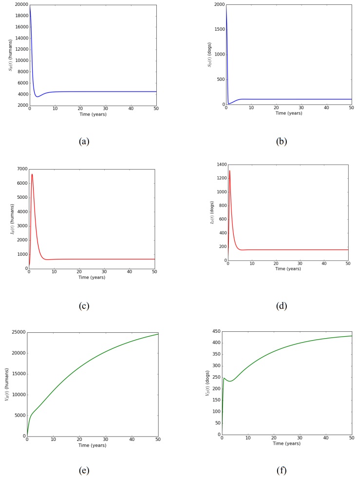
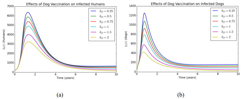
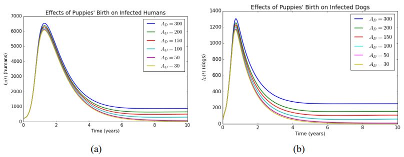
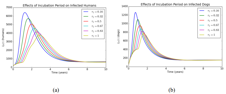
In this article, a delay differential equations model is constructed to observe the spread of rabies among human and dog populations by considering two delay effects on incubation period and vaccine efficacy. Other parameters that affect the spread of rabies are also analyzed. Using the basic reproduction number, it is shown that dog populations and the two delays gives a significant effect on the spread of rabies among human and dog populations. The existence of two delays causes the system to experience Transcritical bifurcation instead of Hopf bifurcation. The numerical simulation shows that depending only on one control method is not enough to reduce or eradicate rabies within the dog populations; instead, it requires several combined strategies, such as increasing dog vaccinations, reducing contact with infected dogs, and controlling puppies' birth. The spread within the human population will be reduced if the spread within the dog population is reduced.
Citation: Muhammad Rifqy Adha Nurdiansyah, Kasbawati, Syamsuddin Toaha. Stability analysis and numerical simulation of rabies spread model with delay effects[J]. AIMS Mathematics, 2024, 9(2): 3399-3425. doi: 10.3934/math.2024167
In this article, a delay differential equations model is constructed to observe the spread of rabies among human and dog populations by considering two delay effects on incubation period and vaccine efficacy. Other parameters that affect the spread of rabies are also analyzed. Using the basic reproduction number, it is shown that dog populations and the two delays gives a significant effect on the spread of rabies among human and dog populations. The existence of two delays causes the system to experience Transcritical bifurcation instead of Hopf bifurcation. The numerical simulation shows that depending only on one control method is not enough to reduce or eradicate rabies within the dog populations; instead, it requires several combined strategies, such as increasing dog vaccinations, reducing contact with infected dogs, and controlling puppies' birth. The spread within the human population will be reduced if the spread within the dog population is reduced.

| [1] | WHO, Rabies, 2023. Available from: https://www.who.int/news-room/fact-sheets/detail/rabies. |
| [2] |
S. Abdulmajid, A. S. Hassan, Analysis of time delayed rabies model in human and dog populations with controls, Afr. Mat., 32 (2021), 1067–1085. https://doi.org/10.1007/s13370-021-00882-w doi: 10.1007/s13370-021-00882-w

|
| [3] |
J. Chen, L. Zou, Z. Jin, S. Ruan, Modeling the geographic spread of rabies in China, PLoS Negl. Trop. Dis., 9 (2015), e0003772. https://doi.org/10.1371/journal.pntd.0003772 doi: 10.1371/journal.pntd.0003772
|
| [4] | Cleveland Clinic, Rabies: causes, symptoms, treatment & prevention, 2022. Available from: https://my.clevelandclinic.org/health/diseases/13848-rabies. |
| [5] | CDC, Animals and rabies, 2022. Available from: https://www.cdc.gov/rabies/animals/index.html. |
| [6] |
A. A. Ayoade, O. J. Peter, T. A. Ayoola, S. Amadiegwu, A. A. Victor, A saturated treatment model for the transmission dynamics of rabies, Malaysian Journal of Computing, 4 (2019), 201–213. https://doi.org/10.24191/mjoc.v4i1.6119 doi: 10.24191/mjoc.v4i1.6119
|
| [7] |
J. Zhang, Z. Jin, G. Q. Sun, T. Zhou, S. Ruan, Analysis of rabies in China: transmission dynamics and control, PLoS ONE, 6 (2011), e20891. https://doi.org/10.1371/journal.pone.0020891 doi: 10.1371/journal.pone.0020891
|
| [8] |
K. Tohma, M. Saito, C. S. Demetria, D. L. Manalo, B. P. Quiambao, T. Kamigaki, et al., Molecular and mathematical modeling analyses of inter-island transmission of rabies into a previously rabies-free island in Philippines, Infect. Genet. Evol., 38 (2016), 22–28. https://doi.org/10.1016/j.meegid.2015.12.001 doi: 10.1016/j.meegid.2015.12.001
|
| [9] |
Y. Huang, M. Li, Application of a mathematical model in determining the spread of the rabies virus: simulation study, JMIR Med. Inform., 8 (2020), e18627. https://doi.org/10.2196/18627 doi: 10.2196/18627
|
| [10] |
B. Pantha, S. Giri, H. R. Joshi, N. K. Vaidya, Modeling transmission dynamics of rabies in Nepal, Infectious Disease Modelling, 6 (2021), 284–301. https://doi.org/10.1016/j.idm.2020.12.009 doi: 10.1016/j.idm.2020.12.009
|
| [11] |
J. K. K. Asamoah, F. T. Oduro, E. Bonyah, B. Seidu, Modelling of rabies transmission dynamics using optimal control analysis, J. Appl. Math., 2017 (2017), 2451237. https://doi.org/10.1155/2017/2451237 doi: 10.1155/2017/2451237
|
| [12] |
M. J. Carroll, A. Singer, G. C. Smith, D. P. Cowan, G. Massei, The use of immunocontraception to improve rabies eradication in urban dog populations, Wildlife Res., 37 (2010), 676–687. https://doi.org/10.1071/WR10027 doi: 10.1071/WR10027
|
| [13] |
C. S. Bornaa, B. Seidu, M. I. Daabo, Mathematical analysis of rabies infection, J. Appl. Math., 2020 (2020), 1804270. https://doi.org/10.1155/2020/1804270 doi: 10.1155/2020/1804270
|
| [14] |
E. K. Renald, D. Kuznetsov, K. Kreppel, Desirable dog-rabies control methods in an urban setting in Africa–a mathematical model, International Journal of Mathematical Sciences and Computing (IJMSC), 6 (2020), 49–67. https://doi.org/10.5815/ijmsc.2020.01.05 doi: 10.5815/ijmsc.2020.01.05
|
| [15] | Q. C. Zhong, Robust control of time-delay systems, London: Springer, 2006. https://doi.org/10.1007/1-84628-265-9 |
| [16] | R. Haberman, Mathematical models: mechanical vibrations, population dynamics, and traffic flow, New Jersey: SIAM, 1998. |
| [17] |
Z. G. Song, J. Xu, Stability switches and double Hopf bifurcation in a two-neural network system with multiple delays, Cogn. Neurodyn., 7 (2013), 505–521. https://doi.org/10.1007/s11571-013-9254-0 doi: 10.1007/s11571-013-9254-0
|
| [18] |
Kasbawati, Y. Jao, N. Erawaty, Dynamic study of the pathogen-immune system interaction with natural delaying effects and protein therapy, AIMS Mathematics, 7 (2022), 7471–7488. https://doi.org/10.3934/math.2022419 doi: 10.3934/math.2022419
|
| [19] | F. Brauer, C. C. Chaves, Mathematical models in population biology and epidemiology, 2 Eds., New York: Springer, 2012. https://doi.org/10.1007/978-1-4614-1686-9 |
| [20] |
O. Diekmann, J. A. P. Heesterbeek, M. G. Roberts, The construction of next-generation matrices for compartmental epidemic models, J. R. Soc. Interface, 7 (2010), 873–885. https://doi.org/10.1098/rsif.2009.0386 doi: 10.1098/rsif.2009.0386
|
| [21] |
R. M. Corless, G. H. Gonnet, D. E. G. Hare, D. J. Jeffrey, D. E. Knuth, On the Lambert W function, Adv. Comput. Math., 5 (1996), 329–359. https://doi.org/10.1007/BF02124750 doi: 10.1007/BF02124750
|
| [22] |
Kasbawati, A. Y. Gunawan, R. Hertadi, K. A. Sidarto, Effects of time delay on the dynamics of a kinetic model of a microbial fermentation process, ANZIAM J., 55 (2014), 336–356. https://doi.org/10.1017/S1446181114000194 doi: 10.1017/S1446181114000194
|
| [23] | S. Wiggins, Introduction to applied nonlinear dynamical systems and chaos, New York: Springer, 1990. https://doi.org/10.1007/978-1-4757-4067-7 |
| [24] |
F. Xu, R. Cressman, Disease control through voluntary vaccination decisions based on the smoothed best response, Comput. Math. Method. M., 2014 (2014), 825734. https://doi.org/10.1155/2014/825734 doi: 10.1155/2014/825734
|
| [25] |
J. Yang, L. Yang, Z. Jin, Optimal strategies of the age-specific vaccination and antiviral treatment against influenza, Chaos Solition. Fract., 168 (2023), 113199. https://doi.org/10.1016/j.chaos.2023.113199 doi: 10.1016/j.chaos.2023.113199
|
| [26] |
F. Xu, R. Cressman, Voluntary vaccination strategy and the spread of sexually transmitted diseases, Math. Biosci., 274 (2016), 94–107. https://doi.org/10.1016/j.mbs.2016.02.004 doi: 10.1016/j.mbs.2016.02.004
|

Figures(10) / Tables(2)

Muhammad Rifqy Adha Nurdiansyah, Kasbawati, Syamsuddin Toaha. Stability analysis and numerical simulation of rabies spread model with delay effects[J]. AIMS Mathematics, 2024, 9(2): 3399-3425. doi: 10.3934/math.2024167


 DownLoad: