Effect of moisture absorption-desorption cycles, UV irradiation and coupling agent on the mechanical performance of pinewood waste/polyethylene composites

Javier Guillén-Mallette; Irma Flores-Cerón; Soledad Cecilia Pech-Cohuo; Edgar José López-Naranjo; Carlos Vidal Cupul-Manzano; Alex Valadez-González; Ricardo Herbé Cruz-Estrada; Javier Guillén-Mallette; Irma Flores-Cerón; Soledad Cecilia Pech-Cohuo; Edgar José López-Naranjo; Carlos Vidal Cupul-Manzano; Alex Valadez-González; Ricardo Herbé Cruz-Estrada

doi:10.3934/ctr.2023013

Clean Technologies and Recycling

2023, Volume 3, Issue 3: 193-220. doi: 10.3934/ctr.2023013

Previous Article Next Article

Research article Topical Sections

Effect of moisture absorption-desorption cycles, UV irradiation and coupling agent on the mechanical performance of pinewood waste/polyethylene composites

1.
Yucatan Scientific Research Center, 130 43rd St., Chuburna de Hidalgo, Merida YU 97205, Mexico
2.
Center for Research and Assistance in Technology and Design of the State of Jalisco, Km 5.5 Sierra Papacal-Chuburna Puerto Highway, Merida YU 97302, Mexico
3.
University Center of Exact Sciences and Engineering, 48 José Guadalupe Zuno, Zapopan JC 45157, Mexico

Received: 25 July 2023 Revised: 05 September 2023 Accepted: 11 September 2023 Published: 20 September 2023

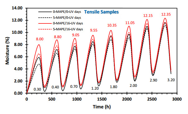
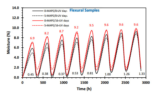
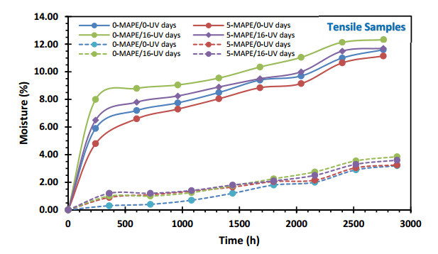
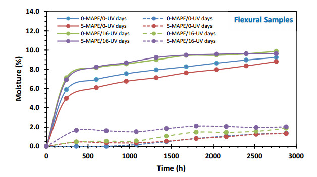
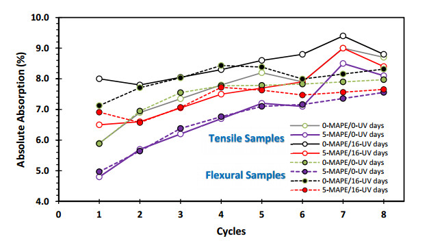
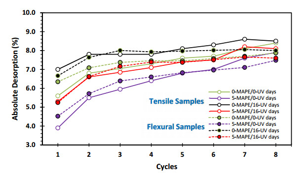
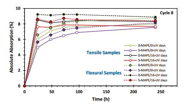
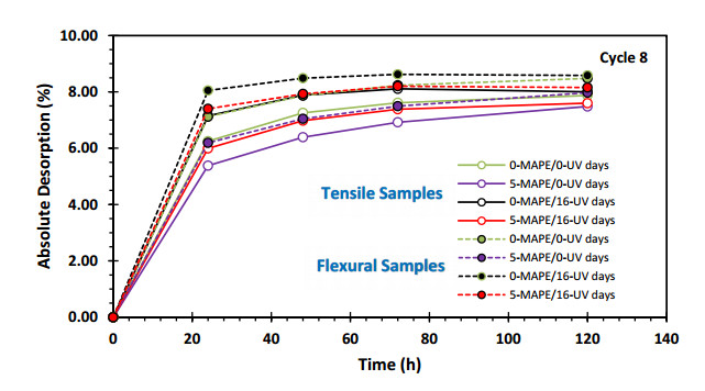
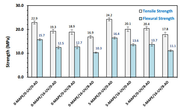
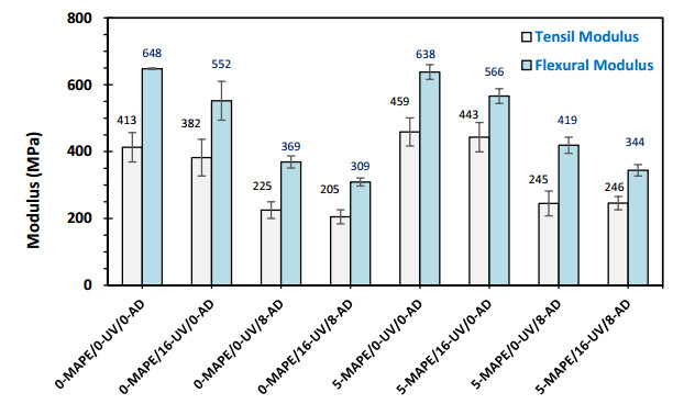
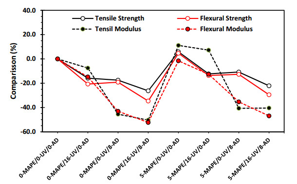
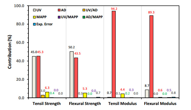
The effects of UV radiation, a maleic anhydride grafted polyethylene (MAPE) coupling agent and moisture cycling exposure on wood plastic composites (WPC) made from pinewood waste (PW) and high-density polyethylene (HDPE) on their tensile and flex properties, were studied. First, the effect of UV radiation and the presence of anhydride grafted polyethylene on the absorption-desorption behavior of the compounds was evaluated and then its effect on the mechanical properties. Scanning electron microscopy (SEM) was used to analyze the surfaces of the samples subjected to these factors and their subsequent damage in fracture zones of the samples. The moisture absorption-desorption process exhibited a two-stage mechanism: the first is significant increases in the absorption values in the first five cycles, and a second stabilization stage that occurs from the sixth cycle onwards. The first stage includes several steps: initial absorption and delamination; capillary action and polymer-wood interaction; and swelling, fiber-matrix interaction and mechanical damage. The second stage involves the balance and stabilization step. Statistically, it was found that the changes in the humidity values in the absorption and desorption cycles show that UV radiation has a significant contribution with the effect of increasing the absorption and desorption values, while the presence of anhydride grafted polyethylene as a lesser effect with an effect of decreasing those values. The tensile and flexural properties of the compounds were significantly affected by UV radiation and moisture cycling. Taking the sample without anhydride grafted polyethylene and without treatments as a reference, only a slight increase of 5–12% in its tensile and flexural properties was observed, while treatments with UV radiation and absorption-desorption cycles reduced them by up to 45%. The SEM analysis confirmed the deterioration of the composites in the form of microcracks, delamination, interfacial voids and mechanical failures in both the wood filler and the polyethylene matrix, especially in the samples exposed to ultraviolet radiation, where this deterioration was lower in the samples containing anhydride grafted polyethylene.
- absorption,
- desorption,
- UV radiation,
- anhydride grafted polyethylene (MAPE),
- cycle,
- moisture,
- wood plastic composite (WPC),
- mechanical properties
Citation: Javier Guillén-Mallette, Irma Flores-Cerón, Soledad Cecilia Pech-Cohuo, Edgar José López-Naranjo, Carlos Vidal Cupul-Manzano, Alex Valadez-González, Ricardo Herbé Cruz-Estrada. Effect of moisture absorption-desorption cycles, UV irradiation and coupling agent on the mechanical performance of pinewood waste/polyethylene composites[J]. Clean Technologies and Recycling, 2023, 3(3): 193-220. doi: 10.3934/ctr.2023013

Related Papers:

Abstract

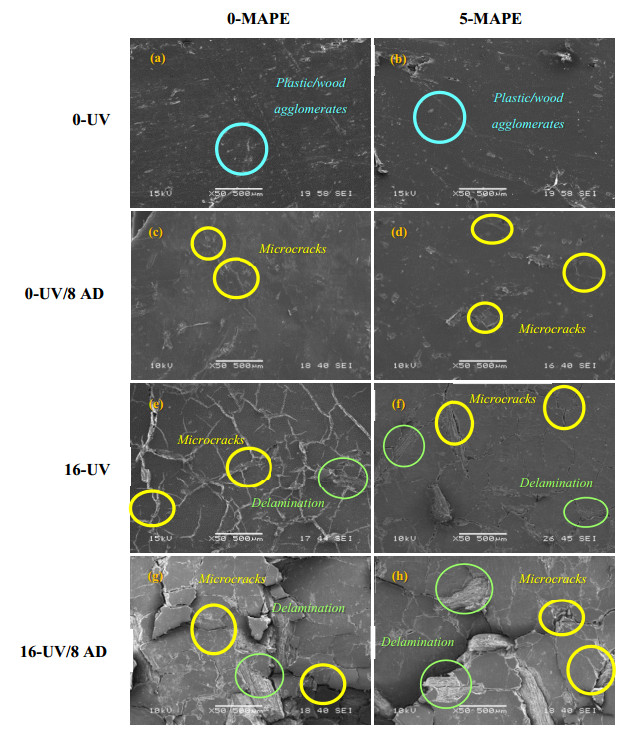
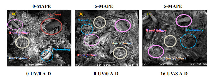
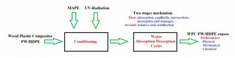
The effects of UV radiation, a maleic anhydride grafted polyethylene (MAPE) coupling agent and moisture cycling exposure on wood plastic composites (WPC) made from pinewood waste (PW) and high-density polyethylene (HDPE) on their tensile and flex properties, were studied. First, the effect of UV radiation and the presence of anhydride grafted polyethylene on the absorption-desorption behavior of the compounds was evaluated and then its effect on the mechanical properties. Scanning electron microscopy (SEM) was used to analyze the surfaces of the samples subjected to these factors and their subsequent damage in fracture zones of the samples. The moisture absorption-desorption process exhibited a two-stage mechanism: the first is significant increases in the absorption values in the first five cycles, and a second stabilization stage that occurs from the sixth cycle onwards. The first stage includes several steps: initial absorption and delamination; capillary action and polymer-wood interaction; and swelling, fiber-matrix interaction and mechanical damage. The second stage involves the balance and stabilization step. Statistically, it was found that the changes in the humidity values in the absorption and desorption cycles show that UV radiation has a significant contribution with the effect of increasing the absorption and desorption values, while the presence of anhydride grafted polyethylene as a lesser effect with an effect of decreasing those values. The tensile and flexural properties of the compounds were significantly affected by UV radiation and moisture cycling. Taking the sample without anhydride grafted polyethylene and without treatments as a reference, only a slight increase of 5–12% in its tensile and flexural properties was observed, while treatments with UV radiation and absorption-desorption cycles reduced them by up to 45%. The SEM analysis confirmed the deterioration of the composites in the form of microcracks, delamination, interfacial voids and mechanical failures in both the wood filler and the polyethylene matrix, especially in the samples exposed to ultraviolet radiation, where this deterioration was lower in the samples containing anhydride grafted polyethylene.

References

[1]	Dolza C, Fages E, Gonga E, et al. (2021) Development and characterization of environmentally friendly wood plastic composites from biobased polyethylene and short natural fibers processed by injection moulding. Polymers 13: 1692. https://doi.org/10.3390/polym13111692 doi: 10.3390/polym13111692
[2]	Pokhrel G, Gardner DJ, Han Y (2021) Properties of wood–plastic composites manufactured from two different wood feedstocks: Wood flour and wood pellets. Polymers 13: 2769. https://doi.org/10.3390/polym13162769 doi: 10.3390/polym13162769
[3]	Yeh S-K, Hu CR, Rizkiana MB, et al. (2021) Effect of fiber size, cyclic moisture absorption and fungal decay on the durability of natural fiber composites. Constr Build Mater 286: 122819. https://doi.org/10.1016/j.conbuildmat.2021.122819 doi: 10.1016/j.conbuildmat.2021.122819
[4]	Al-Maharma AY, Al-Huniti N (2019) Critical review of the parameters affecting the effectiveness of moisture absorption treatments used for natural composites. J Compos Sci 3: 27. https://doi.org/10.3390/jcs3010027 doi: 10.3390/jcs3010027
[5]	Fu H, Dun M, Wang H, et al. (2020) Creep response of wood flour-high-density polyethylene/laminated veneer lumber coextruded composites. Constr Build Mater 237: 117499. https://doi.org/10.1016/j.conbuildmat.2019.117499 doi: 10.1016/j.conbuildmat.2019.117499
[6]	Huang CW, Yang TC, Wu TL, et al. (2018) Effects of maleated polypropylene content on the extended creep behavior of wood-polypropylene composites using the stepped isothermal method and the stepped isostress method. Wood Sci Technol 52: 1313–1330. https://doi.org/10.1007/s00226-018-1037-7 doi: 10.1007/s00226-018-1037-7
[7]	Brebu M (2020) Environmental degradation of plastic composites with natural fillers—A review. Polymers 12: 166. https://doi.org/10.3390/polym12010166 doi: 10.3390/polym12010166
[8]	Benthien JT, Riegler M, Engehausen N, et al. (2020) Specific dimensional change behavior of laminated beech veneer lumber (baubuche) in terms of moisture absorption and desorption. Fibers 8: 47. https://doi.org/10.3390/fib8070047 doi: 10.3390/fib8070047
[9]	Musthaq MA, Dhakal HN, Zhang Z, et al. (2023) The effect of various environmental conditions on the impact damage behaviour of natural-fibre-reinforced composites (NFRCs)—A critical review. Polymers 15: 1229. https://doi.org/10.3390/polym15051229 doi: 10.3390/polym15051229
[10]	Azwa ZN, Yousif BF, Manalo AC, et al. (2013) A review on the degradability of polymeric composites based on natural fibres. Mater Design 47: 424–442. https://doi.org/10.1016/j.matdes.2012.11.025 doi: 10.1016/j.matdes.2012.11.025
[11]	Srubar WV, Billington SL (2013) A micromechanical model for moisture-induced deterioration in fully biorenewable wood–plastic composites. Compos Part A-Appl S 50: 81–92. https://doi.org/10.1016/j.compositesa.2013.02.001 doi: 10.1016/j.compositesa.2013.02.001
[12]	Pech-Cohuo SC, Flores-Cerón I, Valadez-González A, et al. (2016) Interfacial shear strength evaluation of pinewood residue/high-density polyethylene composites exposed to UV radiation and moisture absorption-desorption cycles. BioResources 11: 3719–3735. https://doi.org/10.15376/biores.11.2.3719-3735 doi: 10.15376/biores.11.2.3719-3735
[13]	ASTM D638-14, Standard Test Method for Tensile Properties of Plastics. ASTM International, 2022. Available from: https://www.astm.org/d0638-14.html.
[14]	ASTM D790-17, Standard Test Methods for Flexural Properties of Unreinforced and Reinforced Plastics and Electrical Insulating Materials. ASTM International, 2017. Available from: https://www.astm.org/d0790-17.html.
[15]	ASTM D4329-21, Standard Practice for Fluorescent Ultraviolet (UV) Lamp Apparatus Exposure of Plastics. ASTM International, 2021. Available from: https://www.astm.org/d4329-21.html.
[16]	ASTM G151-19, Standard Practice for Exposing Nonmetallic Materials in Accelerated Test Devices that Use Laboratory Light Sources. ASTM International, 2019. Available from: https://www.astm.org/g0151-19.html.
[17]	ASTM G154-23, Standard Practice for Operating Fluorescent Ultraviolet (UV) Lamp Apparatus for Exposure of Materials. ASTM International, 2023. Available from: https://www.astm.org/g0154-23.html.
[18]	ASTM D618-21, Standard Practice for Conditioning Plastics for Testing. ASTM International, 2021. Available from: https://www.astm.org/d0618-21.html.
[19]	ASTM G147-17, Standard Practice for Conditioning and Handling of Nonmetallic Materials for Natural and Artificial Weathering Tests. ASTM International, 2017. Available from: https://www.astm.org/g0147-17.html.
[20]	ASTM D5229/D5229M-20, Standard Test Method for Moisture Absorption Properties and Equilibrium Conditioning of Polymer Matrix Composite Materials. ASTM International, 2020. Available from: https://www.astm.org/d5229_d5229m-20.html.
[21]	ASTM D570-22, Standard Test Method for Water Absorption of Plastics. ASTM International, 2022. Available from: https://www.astm.org/d0570-22.html.
[22]	Ranjbarha Z, Aberoomand-Azar P, Mokhtari-Aliabad J, et al. (2021) High density polyethylene/wood flour composite: Optimization of processing temperature, processing time and coupling agent concentration. Polym Polym Compos 29: S106–S116. https://doi.org/10.1177/0967391120987338 doi: 10.1177/0967391120987338
[23]	Hao X, Xu J, Zhou H, et al. (2021) Interfacial adhesion mechanisms of ultra-highly filled wood fiber/polyethylene composites using maleic anhydride grafted polyethylene as a compatibilizer. Mater Design 212: 110182. https://doi.org/10.1016/j.matdes.2021.110182 doi: 10.1016/j.matdes.2021.110182
[24]	Adebayo GO (2022) Mechanical and water kinetic parameters of water-absorbed hard wood dust/high-density polyethylene composites. Polymer Bulletin 79: 193–211. https://doi.org/10.1007/s00289-020-03496-7 doi: 10.1007/s00289-020-03496-7
[25]	Krehula LK, Katančić Z, Siročić AP, et al. (2013) Weathering of high-density polyethylene-wood plastic composites. J Wood Chem Technol 34: 39–54. https://doi.org/10.1080/02773813.2013.827209 doi: 10.1080/02773813.2013.827209
[26]	Kallbom S, Lillqvist K, Spoljaric S, et al. (2020) Effects of water soaking-drying cycles on thermally modified spruce wood-plastic composites. Wood Fiber Sci 52: 2–12. https://doi.org/10.22382/wfs-2020-002 doi: 10.22382/wfs-2020-002
[27]	Placette MD, Fan X, Zhao JH, et al. (2012) Dual stage modeling of moisture absorption and desorption in epoxy mold compounds. Microelectron Reliab 52: 1401–1408. https://doi.org/10.1016/j.microrel.2012.03.008 doi: 10.1016/j.microrel.2012.03.008
[28]	Bao LR, Yee AF, Lee CYC (2001) Moisture absorption and hygrothermal aging in a bismaleimide resin. Polymer 42: 7327–7333. https://doi.org/10.1016/S0032-3861(01)00238-5 doi: 10.1016/S0032-3861(01)00238-5
[29]	Pemex Etileno, High density polyethylene, grade 56035 (bimodal). DDR, 2017. Available from: https://donramis.com.mx/productos/.

Reader Comments

Your name:*

Email:*
© 2023 the Author(s), licensee AIMS Press. This is an open access article distributed under the terms of the Creative Commons Attribution License (http://creativecommons.org/licenses/by/4.0)