DNA kinks behavior in the potential pit-trap

Larisa A. Krasnobaeva; Ludmila V. Yakushevich; Larisa A. Krasnobaeva; Ludmila V. Yakushevich

doi:10.3934/biophy.2022012

AIMS Biophysics

2022, Volume 9, Issue 2: 130-146. doi: 10.3934/biophy.2022012

Previous Article Next Article

Research article Special Issues

DNA kinks behavior in the potential pit-trap

Larisa A. Krasnobaeva ^1,2,
Ludmila V. Yakushevich ^{3
,
,}

1.
Siberian State Medical University, 634050 Tomsk, Moscow traсt 2, Russia
2.
Tomsk State University, 634050 Tomsk, Lenin Avenue 36, Russia
3.
Institute of Cell Biophysics, Russian Academy of Sciences, 142290 Pushchino. Institutskaya str. 3, Moscow region, Russia

Received: 10 May 2022 Revised: 31 May 2022 Accepted: 07 June 2022 Published: 10 June 2022

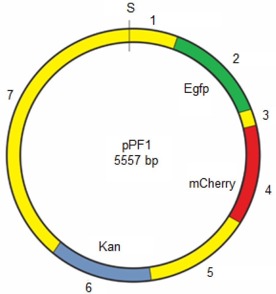
For better understanding the role of dynamic factors in the DNA functioning, it is important to study the internal mobility of DNA and, in particular, the movement of nonlinear conformational distortions -kinks along the DNA chains. In this work, we study the behavior of the kinks in the pPF1 plasmid containing two genes of fluorescent proteins (EGFP and mCherry). To simulate the movement, two coupled nonlinear sine-Gordon equations that describe the angular oscillations of nitrogenous bases in the main and complementary chains and take into account the effects of dissipation and the action of a constant torsion field. To solve the equations, approximate methods such as the quasi-homogeneous approximation, the mean field method, and the block method, were used. The obtained solutions indicate that two types of kinks moving along the double strand can be formed in any part of the plasmid. The profiles of the potential fields in which these kinks are moving are calculated. The results of the calculations show that the lowest energy required for the kink formation, corresponds to the region located between the genes of green and red proteins (EGFP and mCherry). It is shown that it is in this region a pit trap is located for both kinks. Trajectories of the kinks in the pit-trap and nearby are constructed. It is shown that there are threshold values of the torsion field, upon reaching which the kinks behavior changes dramatically: there is a transition from cyclic motion inside the pit-trap to translational motion and exit from the potential pit-trap.

Keywords:

Citation: Larisa A. Krasnobaeva, Ludmila V. Yakushevich. DNA kinks behavior in the potential pit-trap[J]. AIMS Biophysics, 2022, 9(2): 130-146. doi: 10.3934/biophy.2022012

Related Papers:

[1]	Ludmila V. Yakushevich, Larisa A. Krasnobaeva . Double energy profile of pBR322 plasmid. AIMS Biophysics, 2021, 8(2): 221-232. doi: 10.3934/biophy.2021016
[2]	Larisa A. Krasnobaeva, Ludmila V. Yakushevich . On the dimensionless model of the transcription bubble dynamics. AIMS Biophysics, 2023, 10(2): 205-219. doi: 10.3934/biophy.2023013
[3]	Delores J. Grant, Leighcraft A. Shakes, Hope M. Wolf, Derek C. Norford, Pradeep K. Chatterjee . Exploring function of conserved non-coding DNA in its chromosomal context. AIMS Biophysics, 2015, 2(4): 773-793. doi: 10.3934/biophy.2015.4.773
[4]	Jacqueline Acres, Jay Nadeau . 2D vs 3D tracking in bacterial motility analysis. AIMS Biophysics, 2021, 8(4): 385-399. doi: 10.3934/biophy.2021030
[5]	Alexander G. Volkov, Yuri B. Shtessel . Propagation of electrotonic potentials in plants: Experimental study and mathematical modeling. AIMS Biophysics, 2016, 3(3): 358-379. doi: 10.3934/biophy.2016.3.358
[6]	Marcelina Cardoso Dos Santos, Cyrille Vézy, Hamid Morjani, Rodolphe Jaffol . Single cell adhesion strength assessed with variable-angle total internal reflection fluorescence microscopy. AIMS Biophysics, 2017, 4(3): 438-450. doi: 10.3934/biophy.2017.3.438
[7]	Tomohiro Yanao, Sosuke Sano, Kenichi Yoshikawa . Chiral selection in wrapping, crossover, and braiding of DNA mediated by asymmetric bend-writhe elasticity. AIMS Biophysics, 2015, 2(4): 666-694. doi: 10.3934/biophy.2015.4.666
[8]	Larisa I. Fedoreyeva, Boris F. Vanyushin . Regulation of DNA methyltransferase gene expression by short peptides in nicotiana tabacum regenerants. AIMS Biophysics, 2021, 8(1): 66-79. doi: 10.3934/biophy.2021005
[9]	Audrey Lejart, Gilles Salbert, Sébastien Huet . Cytosine hydroxymethylation by TET enzymes: From the control of gene expression to the regulation of DNA repair mechanisms, and back. AIMS Biophysics, 2018, 5(3): 182-193. doi: 10.3934/biophy.2018.3.182
[10]	Larisa I. Fedoreyeva, Tatiana A. Dilovarova, Boris F. Vanyushin, Inna A. Chaban, Neonila V. Kononenko . Regulation of gene expression in Nicotiana tabacum seedlings by the MKASAA peptide through DNA methylation via the RdDM pathway. AIMS Biophysics, 2022, 9(2): 113-129. doi: 10.3934/biophy.2022011

Abstract

1. Introduction

Dynamics is known to play an important role in the functioning of DNA. Despite this, many questions regarding the features of the internal DNA mobility as well as their connection with the functioning are still unclear. In this work, we investigate the dynamic behavior of the nonlinear conformational distortions—DNA kinks [1], which are small locally unwound regions of the double helix, also named open states [2] or, in later works, bubbles [3]–[5] or transcription bubbles [6]–[9]. We study in detail the DNA kinks movement in the potential field containing a pit-trap. These traps are often found in the potential fields of small circular plasmids.

Plasmids are widely used in genetic engineering to study the functional properties of DNA molecules and its fragments. In recent years, plasmids containing genes for fluorescent proteins have been especially actively used. By inserting the studied DNA fragments into the intermediate region between two genes of fluorescent proteins, for example, between the genes of green and red proteins (EGFP [10] and mCherry [11]), researchers judge the intensity and direction of the transcription process in these DNA fragments according to the fluorescence spectra.

To carry out model experiments, we chose the recently created pPF1 plasmid containing a pit trap. This plasmid (Figure 1) was constructed by Masulis et al. in 2015 [12]. It was obtained from the pET-28b plasmid [13] and supplemented with two genes: EGFP and mCherry, encoding green and red fluorescent proteins, respectively. The complete nucleotide sequence of pPF1 was published in 2021 in the work of Masulis et al. [14] (see the sequence in Appendix where the region between the two genes is underlined).

Figure 1. Schematic representation of the plasmid pPF1. The gene EGFP, the gene mCherry and the kanamycin resistance gene are shown in green, red and blue, respectively. Intermediate regions are shown in yellow. S indicates the beginning of the numbering of the nucleotide sequence. The numbers 1, 2, 3, 4, 5, 6 and 7 number the regions.

DownLoad: Full-Size Img PowerPoint

For mathematical modeling of the plasmid structure, it is convenient to renumber sequentially the sections of the sequence corresponding to these three genes and intermediate regions between them, starting from point S (Figure 1). As a result, we get 7 regions. However, when performing mathematical calculations, it its necessary to take into account the circular nature of the plasmid structure. To do this, it is convenient to combine the regions to the right and left of the point S (the 1-st and 7-th regions) into a single region and call it the (7 + 1)-th region. Data on the coordinates of the regions, the number of adenines N_A, thymines N_T, guanines N_G and cytosines N_C and the total number of bases in each region are presented in Table 1.

Table 1. Details оf the plasmid pPF1 structure.

Region number	Region coordinates	N_A	N_T	N_G	N_C	N
1+7	(1-332) + (3382-5557)	549	582	709	668	2508
2 (EGFP)	333..1049	102	172	240	203	717
3	1050-1133	28	28	14	14	84
4 (mCherry)	1134-1841	163	100	220	225	708
5	1842-2568	168	208	165	186	727
6 (Kan)	2569-3381	247	210	162	194	813

| Show Table

DownLoad: CSV

Figure 2. Fragment of the pPF1 plasmid nucleotide sequence containing the 3-rd region. Red and green markers highlight the genes of red and green proteins, respectively. The yellow color shows the intermediate region between the genes.

DownLoad: Full-Size Img PowerPoint

The structure of the 3-rd (intermediate) region is of special attention. It consists of two parts equal in length, and the sequence of the second part is complementary and inverted with respect to the sequence of the first part. A fragment of the plasmid sequence containing the genes of green and red proteins, as well as the intermediate region between them, is shown in Figure 2. Protein genes are highlighted with green and red markers and the intermediate region with yellow marker.

To study the behavior of kinks in the 3-rd region, we chose the McLaughlin-Scott method [15],[16] with an improved and adapted for DNA algorithm for calculating the dynamic characteristics of kinks [17]. The results of the study will be presented in the form of calculated 2D and 3D trajectories of DNA kinks.

2. Model and methods

There are many mathematical models that are applied to imitate DNA internal mobility and elucidate the role of the internal dynamics in the DNA functioning, in the DNA-environment and DNA-DNA interactions [18]–[20]. In this work, we use the model based on the assumption that the main contribution to the opening of pairs of nitrogenous bases and the formation of open states is made by the angular deviations of nitrogenous bases from equilibrium positions (Figure 3). To describe the deviations, the Englander model [2] or its modifications which allow solutions in the form of local conformational distortions (solitary waves or solitons) moving along the DNA double strand, are often used. Here we use modification that takes into account the deviations of bases, both in the main and complementary DNA strands, and the effects of dissipation and the action of a constant torsion moment M₀:

$\begin{array}{l} I_{n, 1} \frac{d^{2} φ_{n, 1} (t)}{d t^{2}} - K_{n, 1}^{'} [φ_{n + 1, 1} (t) - 2 φ_{n, 1} (t) + φ_{n - 1, 1} (t)] + \\ + k_{n, 1 - 2} R_{n, 1} (R_{n, 1} + R_{n, 2}) \sin φ_{n, 1} (t) - k_{n, 1 - 2} R_{n, 1} R_{n, 2} \sin (φ_{n, 1} (t) - φ_{n, 2} (t)) = \\ = - β_{n, 1} \frac{d φ_{n, 1} (t)}{d t} + M_{0}, \end{array}$ (1)

$\begin{array}{l} I_{n, 2} \frac{d^{2} φ_{n, 2} (t)}{d t^{2}} - K_{n, 2}^{'} [φ_{n + 1, 2} (t) - 2 φ_{n, 2} (t) + φ_{n - 1, 2} (t)] + \\ + k_{n, 1 - 2} R_{n, 2} (R_{n, 1} + R_{n, 2}) \sin φ_{n, 2} (t) - k_{n, 1 - 2} R_{n, 1} R_{n, 2} \sin (φ_{n, 2} (t) - φ_{n, 1} (t)) = \\ = - β_{n, 2} \frac{d φ_{n, 2} (t)}{d t} + M_{0} . \end{array}$ (2)

Here $φ_{n, i} (t)$ is the angular deviation of the n-th nitrogenous base in the i-th chain of one of the six regions of the plasmid; $I_{n, i}$ is the moment of inertia of the n-th nitrogenous base of the i-th chain; $R_{n, i}$ is the distance from the center of mass of the n-th nitrogenous base of the i-th chain to the sugar-phosphate backbone; $K_{n, 1}^{'} = K R_{n, i}^{2}$ ; K is the rigidity of the sugar-phosphate backbone; $β_{n, i} = α R_{n, i}^{2}$ ; α is the dissipation coefficient; $k_{n, i}$ is a constant characterizing the interaction between bases within pairs; i = 1, 2; n = 1, 2, ... N, N is the total number of bases in the region under consideration; $M_{0}$ is a constant external moment. An example of this type of moment is the torsion moment resulting from the interaction of RNA polymerase with the promoter region of DNA at the initial stage of transcription.

In contrast to the equations used in our previous work [21], modification (1)–(2) takes into account the influence of the torsion moment $M_{0}$ on the movement of local conformational distortions along the DNA double strand.

Figure 3. Schematic representation of a DNA double strand fragment. $φ_{n, 1}$ is the angular deviation of the n-th nitrogenous base in the 1-st chain, $φ_{n, 2}$ is the angular deviation of the n-th nitrogenous base in the 2-nd chain. $R_{n + 1, 1}$ is the distance from the center of mass of the (n+1)-st nitrogenous base to the 1-st sugar-phosphate chain and $R_{n + 1, 2}$ is the distance from the center of mass of the (n+1)-st nitrogenous base to the 2-nd sugar-phosphate chain; a is the distance between the nearest base pairs.

DownLoad: Full-Size Img PowerPoint

To simplify the solution of problem (1)–(2), we average the coefficients of the equations within each of the 6 regions of the pPF1 plasmid according to formulas:

$\begin{array}{l} I_{n, i} \to {\bar{I}}_{i} = I_{A} C_{A, i} + I_{T} C_{T, i} + I_{G} C_{G, i} + I_{C} C_{C, i}, \\ R_{n, i} \to {\bar{R}}_{i} = R_{A} C_{A, i} + R_{T} C_{T, i} + R_{G} C_{G, i} + R_{C} C_{C, i}, \\ K_{n, i}^{'} \to {\bar{K}}_{i}^{'} = K_{A}^{'} C_{A, i} + K_{T}^{'} C_{T, i} + K_{G}^{'} C_{G, i} + K_{C}^{'} C_{C, i} . \\ k_{n, 1 - 2} \to {\bar{k}}_{1 - 2} = k_{A - T} (C_{A, 1} + C_{T, 2}) + k_{G - C} (C_{G, 1} + C_{C, 2}), \\ β_{n, i} \to {\bar{β}}_{i} = β_{A} C_{A, i} + β_{T} C_{T, i} + β_{G} C_{G, i} + β_{C} C_{C, i}, \end{array}$ (3)

where C_j,i = N_j,i/N; N_j,i is the number of bases of the j-th type (j = А, Т, G, С) of the i-th chain (i = 1, 2) in the region considered. Formulas (3) contain the dynamic parameters that are pertinent to real DNA molecules. The values of the parameters are presented in the Table 2.

Table 2. DNA dynamic parameters [17].

Type of the base in the sequence	I (10⁻⁴⁴ kg∙m²)	K/(10⁻¹⁸ J)	R (10⁻¹⁰ m)	k_1-2 (10⁻² N/m)	β (J∙s)
А	7.61	2.35	5.80	6.20	4.25
Т	4.86	1.61	4.80	6.20	2.91
G	8.22	2.27	5.70	9.60	4.10
C	4.11	1.54	4.70	9.60	2.79

| Show Table

DownLoad: CSV

Then we apply the continuum approximation, which is valid if the solutions we are looking for are smooth. The resulting equations take the form:

$\begin{array}{l} {\bar{I}}_{1} φ_{1, t t} - {\bar{K}}_{1}^{'} a^{2} φ_{1, z z} + {\bar{k}}_{1 - 2} {\bar{R}}_{1} ({\bar{R}}_{1} + {\bar{R}}_{2}) \sin φ_{1} - \\ - {\bar{k}}_{1 - 2} {\bar{R}}_{1} {\bar{R}}_{2} \sin (φ_{1,} - φ_{2}) = - {\bar{β}}_{1} φ_{1, t} + M_{0}, \end{array}$ (4)

$\begin{array}{l} {\bar{I}}_{2} φ_{2, t t} - {\bar{K}}_{2}^{'} a^{2} φ_{2, z z} + {\bar{k}}_{1 - 2} {\bar{R}}_{1} ({\bar{R}}_{1} + {\bar{R}}_{2}) \sin φ_{2} - \\ - {\bar{k}}_{1 - 2} {\bar{R}}_{1} {\bar{R}}_{2} \sin (φ_{2} - φ_{1}) = - {\bar{β}}_{2} φ_{2, t} + M_{0} . \end{array}$ (5)

Taking into account the distribution of interactions within the DNA molecule, namely “weak” hydrogen bonds between nitrogenous bases within complementary pairs and “strong” valence interactions along sugar-phosphate chains, we apply the mean field approximation. As a result, instead of two coupled equations (4)–(5), we obtain two independent equations:

${\bar{I}}_{1} φ_{1, t t} - {\bar{K}}_{1}^{'} a^{2} φ_{1, z z} + {\bar{k}}_{1 - 2} {\bar{R}}_{1}^{2} \sin φ_{1} = - {\bar{β}}_{1} φ_{1. t} + M_{0},$ (6)

${\bar{I}}_{2} φ_{2. t t} - {\bar{K}}_{2}^{'} a^{2} φ_{2, . z z} + {\bar{k}}_{1 - 2} {\bar{R}}_{2}^{2} \sin φ_{2} = - {\bar{β}}_{2} φ_{2, t} + M_{0} .$ (7)

The first equation imitates the angular deviations of the bases in the main chain. The second describes the angular deviations of the bases in the complementary chain.

In the particular case ${\bar{β}}_{1} = 0$ and $M_{0} = 0$ , the first equation reduces to a simple sine-Gordon equation:

${\bar{I}}_{1} φ_{1, t t} - {\bar{K}}_{1}^{'} a^{2} φ_{1, z z} + {\bar{V}}_{1} \sin φ_{1} = 0,$ (8)

whose one-soliton solution - kink, has the form:

$φ_{k, 1} (z, t) = 4 arctg {\exp [({\bar{γ}}_{1} / {\bar{d}}_{1}) (z - {\bar{υ}}_{k, 1} (t) ∙ t - z_{0, 1})]}$ (9)

Here ${\bar{υ}}_{k, 1} (t)$ is the kink velocity in the main chain; ${\bar{γ}}_{1} = {(1 - {\bar{υ}}_{k, 1}^{2} / {\bar{C}}_{1}^{2})}^{- 1 / 2}$ is the Lorentz factor; ${\bar{C}}_{1} = {({\bar{K}}_{1}^{'} a^{2} / {\bar{I}}_{1})}^{1 / 2}$ is the sound velocity; ${\bar{V}}_{1} = {\bar{k}}_{1 - 2} {\bar{R}}_{1}^{2}$ ; ${\bar{d}}_{1} = {({\bar{K}}_{1}^{'} a^{2} / {\bar{V}}_{1})}^{1 / 2}$ is the kink size; $z_{0, 1}$ is the kink coordinate at the initial moment of time. The total energy and rest energy of the kink (9) are determined by the following formulas:

${\bar{E}}_{1} = {\bar{E}}_{0, 1} ∙ {\bar{γ}}_{1},$ (10)

${\bar{E}}_{0, 1} = 8 \sqrt{{\bar{K}}_{1}^{'} {\bar{V}}_{1}} .$ (11)

In the general case ( ${\bar{β}}_{1} \neq 0,$ $M_{0} \neq 0$ ), an exact analytical solution of equation (6) has not yet been found. The approximate solution found by the McLaughlin-Scott method has the form [17]:

${\bar{υ}}_{k, 1} (t) = \frac{[({\bar{υ}}_{0, 1} {\bar{γ}}_{0, 1} - \frac{{\bar{C}}_{1} M_{0} π}{4 {\bar{β}}_{1}} \sqrt{\frac{{\bar{I}}_{1}}{{\bar{V}}_{1}}}) \exp (- \frac{{\bar{β}}_{1}}{{\bar{I}}_{1}} (t - t_{0})) + \frac{{\bar{C}}_{1} M_{0} π}{4 {\bar{β}}_{1}} \sqrt{\frac{{\bar{I}}_{1}}{{\bar{V}}_{1}}}]}{\sqrt{1 + {[(\frac{{\bar{υ}}_{0, 1}}{{\bar{C}}_{1}} {\bar{γ}}_{0, 1} - \frac{M_{0} π}{4 {\bar{β}}_{1}} \sqrt{\frac{{\bar{I}}_{1}}{{\bar{V}}_{1}}}) \exp (- \frac{{\bar{β}}_{1}}{{\bar{I}}_{1}} (t - t_{0})) + \frac{M_{0} π}{4 {\bar{β}}_{1}} \sqrt{\frac{{\bar{I}}_{1}}{{\bar{V}}_{1}}}]}^{2}}},$ (12)

where $t_{0}$ is the start time of the first kink; ${\bar{υ}}_{0, 1}$ is the initial kink velocity; ${\bar{γ}}_{0, 1} = {(1 - {\bar{υ}}_{0, 1}^{2} / {\bar{C}}_{1}^{2})}^{- 1 / 2}$ . The approximate solution of the second equation (namely, equation (7)), found in a similar way, has the form:

$φ_{k, 2} (z, t) = 4 arctg {\exp [({\bar{γ}}_{2} / {\bar{d}}_{2}) (z - {\bar{υ}}_{k, 2} (t) ∙ t - z_{0, 2})]},$ (13)

where ${\bar{υ}}_{k, 2} (t)$ is the kink velocity in the complementary chain; ${\bar{γ}}_{2} = {(1 - {\bar{υ}}_{k, 2}^{2} / {\bar{C}}_{2}^{2})}^{- \frac{1}{2}}$ is the Lorentz factor; ${\bar{C}}_{2} = {({\bar{K}}_{2}^{′} a^{2} / {\bar{I}}_{2})}^{1 / 2}$ is the sound velocity; ${\bar{V}}_{2} = {\bar{k}}_{1 - 2} {\bar{R}}_{2}^{2}$ ; ${\bar{d}}_{2} = {({\bar{K}}_{2}^{′} a^{2} / {\bar{V}}_{2})}^{1 / 2}$ is the kink size; $z_{0, 2}$ is the kink coordinate at the initial moment of time. The total energy and rest energy of the kink (13) are determined by the following formulas:

${\bar{E}}_{2} = {\bar{E}}_{0, 2} ∙ {\bar{γ}}_{2},$ (14)

${\bar{E}}_{0, 2} = 8 \sqrt{{\bar{K}}_{2}^{'} {\bar{V}}_{2}} .$ (15)

The kink velocity is equal to:

${\bar{υ}}_{k, 2} (t) = \frac{[({\bar{υ}}_{0, 2} {\bar{γ}}_{0, 2} - \frac{{\bar{C}}_{2} M_{0} π}{4 {\bar{β}}_{2}} \sqrt{\frac{{\bar{I}}_{2}}{{\bar{V}}_{2}}}) \exp (- \frac{{\bar{β}}_{2}}{{\bar{I}}_{2}} (t - t_{0})) + \frac{{\bar{C}}_{2} M_{0} π}{4 {\bar{β}}_{2}} \sqrt{\frac{{\bar{I}}_{2}}{{\bar{V}}_{2}}}]}{\sqrt{1 + {[(\frac{{\bar{υ}}_{0, 2}}{{\bar{C}}_{2}} {\bar{γ}}_{0, 2} - \frac{M_{0} π}{4 {\bar{β}}_{2}} \sqrt{\frac{{\bar{I}}_{2}}{{\bar{V}}_{2}}}) \exp (- \frac{{\bar{β}}_{2}}{{\bar{I}}_{2}} (t - t_{0})) + \frac{M_{0} π}{4 {\bar{β}}_{2}} \sqrt{\frac{{\bar{I}}_{2}}{{\bar{V}}_{2}}}]}^{2}}},$ (16)

where ${\bar{υ}}_{0, 2}$ is the initial velocity; ${\bar{γ}}_{0, 2} = {(1 - {\bar{υ}}_{0, 2}^{2} / {\bar{C}}_{2}^{2})}^{- 1 / 2}$ .

Thus, within the framework of the approximation described above, in any DNA regions, two types of kinks: $φ_{k, 1} (z, t)$ and $φ_{k, 2} (z, t)$ , can be formed. Moreover, they can be interpreted as quasiparticles moving along the DNA double strand.

3. Results and discussion

3.1. Profile of the potential field where the first kink moves

To construct the profile of the potential field in which the kink defined by formula (9), moves, the averaged values of the coefficients ${\bar{I}}_{1}, {\bar{K'}}_{1}, {\bar{V}}_{1}$ and the rest energy ${\bar{E}}_{0, 1}$ were calculated for each region of the main sequence. The calculation results are presented in Table 3, and the corresponding energy profile is shown in Figure 4a.

Table 3. Averaged values of the coefficients ${\bar{I}}_{1}, {\bar{K'}}_{1}, {\bar{V}}_{1}$ and the rest energy ${\bar{E}}_{0, 1}$ calculated for each region of the main plasmid pPF1 sequence.

Region number	I₁×10^-44 (kg·m²)	K′₁×10^-18 (N·m)	V₁×10^-20 (J)	E_0,1×10^-18 (J)
1 + 7	6.21	1.94	2.23	1.67
2 (EGFP)	6.16	1.92	2.28	1.67
3	6.21	1.96	2.04	1.60
4 (mCherry)	6.30	1.96	2.32	1.71
5	6.06	1.91	2.14	1.62
6 (Kan)	6.18	1.95	2.13	1.63

| Show Table

DownLoad: CSV

Figure 4. Profile of the potential field where the first kink moves (a) and schematic presentation of the plasmid pPF1 sequence cut at point S and expanded into a line (b). The red small star symbolizes the kink. The arrow indicates the direction of kink movement. Vertical gray lines indicate the boundaries of the regions. ${\bar{E}}_{0, 1}^{(2)}$ and ${\bar{E}}_{0, 1}^{(4)}$ are the heights of the energy barriers that are located in the 2-nd and 4-th sections of the main plasmid sequence.

DownLoad: Full-Size Img PowerPoint

From Figure 4a it can be seen that the potential field where the kink moves really contains a pit-trap located between the genes of the green and red proteins (Figure 4b). The formation of the kink in this region requires the least amount of energy. Therefore, when simulating the motion of this kink, we assume that at the initial moment the kink is activated in the pit-trap. For definiteness, we suggest that the starting point is located in the center of the pit-trap ( $z_{0, 1} = 1092 bp$ ), the starting velocity ${\bar{υ}}_{0, 1}$ is equal to zero and the torsion moment М0 is directed from 5′ to 3′ end of the main sequence.

From Figure 4 it can be seen also that the movement of the kink will be hindered by an energy barrier located to the right of the pit-trap. To overcome this barrier and continue moving, the following condition must

${\bar{E}}_{0, 1}^{(3)} ∙ γ_{0, 1}^{(3)} \geq {\bar{E}}_{0, 1}^{(4)}$ (17)

where additional superscripts that indicate the region number, are introduced.

From condition (17), we obtain formula for calculating the threshold value of the kink velocity:

$υ_{c r i t, r i g h t} = {\bar{С}}_{1}^{(3)} \sqrt{1 - {(\frac{{\bar{E}}_{0, 1}^{(3)}}{{\bar{E}}_{0, 1}^{(4)}})}^{2}}$ (18)

Inserting the values of the parameters gathered in Table 3 into formula (12), we find the threshold velocity $υ_{c r i t, r i g h t}$ = 673.25 m/s. This velocity value corresponds to the threshold value of the moment $M_{0, c r i t, r i g h t}$ = 4.95×10^-22 J.

3.2. First kink behavior in the case M₀ < M_0,crit,right

Figure 5 illustrates the behavior of the first kink in the case M₀ = 2.50×10^-22 J which is less than M_0,crit,right. The time dependence of the kink velocity is presented in Figure 5a. For convenience, we divided the timeline into several intervals in accordance with the character of the kink behavior and used different colors for different intervals.

Figure 5. Time dependence of the velocity (a) and coordinate (b) of the first kink. The kink trajectory on the phase plane {v, z} (c) and the kink 3D trajectory (d). M₀ = 2.50×10^-22 J, ${\bar{υ}}_{0, 1} =$ 0, z_0,1 = 1092 bp. The segments of the curves corresponding to the time interval (0; 5.45×10^-11 s) are highlighted in brown, those corresponding to the time interval (5.45×10^-11 s; 1.42×10^-10 s) are highlighted in blue, those corresponding to the time interval (1.42×10^-10 s; 2.16×10^-10 s) are highlighted in red.

DownLoad: Full-Size Img PowerPoint

Having determined the kink coordinate by the formula:

$υ_{k, 1} = \frac{d z_{k, 1}}{d t},$ (19)

we obtained the time dependence of the kink coordinate (Figure 5b), as well as the kink trajectory on the phase plane {υ_{k,1, Zk,1}} (Figure 5c) and in the three-dimensional space {υ_{k,1, Zk,1}, t} (Figure 5d).

From Figure 5b, it can be seen that the kink, having started moving from the center of the 3-rd section, reaches the right boundary z_rb = 1133 bp) at the time t_rb = 5.45×10^-11 s. Inserting this value of time into formula (11), we found the kink velocity at the right boundary: υ_rb = 476.73 m/s. It turned out that this value was less than the threshold velocity υ_crit,right = 673.25 m/s. Therefore, the kink could not overcome the right boundary and was reflected from it. This is clearly seen in graphs 5a, b, d (brown segments of curves). It is also clearly seen that the motion of the kink in the time interval (0;5.45×10^-11 s) is divided into two stages: a smooth movement to the right boundary and a sharp reflection from it, which corresponds to a sharp vertical drop in the velocity down on graphs 5a and 5c. The velocity at this moment changes from a value of 476.73 m/s to a value of 476.73 m/s.

Then the kink again begins to move smoothly (blue segments of the curves), but in the opposite direction. It can be seen from Figures 5a,b,d that, having passed part of the way in the direction of the left boundary, the kink smoothly turns back to the right boundary. By the time moment of 1.42×10^-10 s, the kink reaches the right boundary and is reflected from it. At the same time moment, the kink velocity sharply drops down from the value of 411.50 m/s to the value of -411.50 m/s.

The next cycle of the kink movement (red segments of the curves) also includes (1) a smooth movement from the right boundary direction the left boundary, (2) a smooth turn by 180° before reaching the left boundary, (3) a smooth movement in the direction of the right boundary, and (4) a sharp reflection from the right boundary. Obviously, such cycles will continue. At the same time, the kink velocity will decrease upon reaching the right boundary and tend to zero in the limit.

3.3. First kink behavior in the case M₀ > M_0,crit,right

Figures 6a and 6b show the time dependences of the first kink velocity and coordinate in the case of M₀ = 2.50×10^-22 J > M_0,crit,right. In Figures 6c and 6d the kink trajectories on the phase plane {υ_k_{,1, Zk,1}} and in the three-dimensional space {υ_k_{,1, Zk,1}, t} are presented.

From the graph of the time dependence of the coordinate presented in Figure 6b, it can be seen that the kink, having started moving from the center of the 3-rd region, reaches the right boundary by the time 3.42×10^-11 s. In this case, the kink velocity at this boundary becomes equal to υ_crit,right = 775.68 m/s. Since this value is greater than the threshold value of the velocity υ_crit,right = 673.25 m/s, the kink overcomes the boundary and enter the 4-th region corresponding to the red protein gene. It can be seen that the behavior of the kink includes three stages: a smooth movement to the right boundary, a sharp vertical drop down to a value of 409.83 m/s at this boundary and a smooth movement in the 4-th region.

Figure 6. Time dependence of the velocity (a) and coordinate (b) of the first kink. The kink trajectory on the phase plane {v, z} (c) and the kink 3D trajectory (d). M₀ = 6.50×10^-22 J, υ_0,1 = 0, z_0,1 = 1092 bp. The segments of curves corresponding to the movement of the kink in the time interval (0; 3.42×10^-11 s) are highlighted in brown, the segments corresponding to the movement in the time interval (3.42×10^-11 s; 2.16×10^-10 s) are highlighted in blue.

DownLoad: Full-Size Img PowerPoint

3.4. Profile of the potential field where the second kink moves

Table 4. Averaged values of the coefficients I₂, K′₂, V₂ and the rest energy E_0,2 calculated for each region of the complementary plasmid pPF1 sequence.

Region number	I₂×10^-44 (kg·m²)	K′₂×10^-18 (N·m)	V₂×10^-20 (J)	E_0,2 ×10^-18 (J)
1+7	6.18	1.94	2.23	1.66
2 (EGFP)	6.22	1.95	2.28	1.69
3	6.21	1.96	2.04	1.60
4 (mCherry)	6.08	1.90	2.27	1.66
5	6.33	1.98	2.21	1.67
6 (Kan)	6.22	1.95	2.14	1.64

| Show Table

DownLoad: CSV

Figure 7. Profile of the potential field where the second kink moves (a), and schematic presentation of the plasmid pPF1 sequence cut at point S and expanded into a line (b). The blue small star symbolizes the second kink. The arrow indicates the direction of the kink movement. Vertical gray lines indicate the boundaries of the regions. ${\bar{E}}_{0, 2}^{(2)}$ and ${\bar{E}}_{0, 2}^{(4)}$ are the heights of the energy barriers that are located in the 2-nd and 4-th regions of the complementary plasmid sequence.

DownLoad: Full-Size Img PowerPoint

To construct the profile of the potential field in which the second kink defined by formula (13), moves, we calculated the averaged values of the coefficients ${\bar{I}}_{2}, {\bar{K'}}_{2}, {\bar{V}}_{2}$ and the rest energy ${\bar{E}}_{0, 2}$ for each region of the complementary sequence. The calculation results are presented in Table 4, and the corresponding energy profile is shown in Figure 7a.

From Figure 7a it can be seen that the potential field where the second kink moves also contains a pit-trap located between the genes of the green and red proteins (Figure 7b). The formation of the kink in this region requires the least amount of energy. When modeling the movement of this second kink, we assume that at the initial moment of time the kink is activated in the center of the pit-trap well (z_0,2=1092 bp) and its initial velocity υ_0,2 is equal to zero.

From Figure 7 it can be seen also that the movement of the second kink will be hindered by an energy barrier located to the left of the pit-trap. To overcome the barrier and continue moving, the following condition must be fulfilled:

${\bar{E}}_{0, 2}^{(3)} ∙ {\bar{γ}}_{0, 2}^{(3)} \geq {\bar{E}}_{0, 2}^{(2)} .$ (20)

Here superscripts indicate the region number.

From condition (20), we obtain formula for calculating the threshold value of the kink velocity:

$υ_{c r i t, l e f t} = {\bar{С}}_{2}^{(3)} \sqrt{1 - {(\frac{{\bar{E}}_{0, 2}^{(3)}}{{\bar{E}}_{0, 2}^{(2)}})}^{2}} .$ (21)

Inserting the values of the parameters gathered in Table 3, into formula (21), we find the threshold velocity υ_crit,left = 627.21 m/s. This velocity value corresponds to the threshold value of the moment M_0,crit,left= 4.20×10^-22 J.

3.5. Second kink behavior

Figure 8. Time dependence of the velocity (a) and coordinate (b) of the second kink. The kink trajectory on the phase plane {v, z} (c) and the kink 3D trajectory (d). M₀ = -2.50×10^-22 J, υ_0,1 = 0, z_0,1 = 1092 bp. The segments of the curves corresponding to the time interval (0; 5.55×10^-11 s) are highlighted in black, those corresponding to the time interval (5.55×10^-11 s; 1.41×10^-10 s) are highlighted in green, those corresponding to the time interval (1.41×10^-10 s; 2.15×10^-10 s) are highlighted in purple.

DownLoad: Full-Size Img PowerPoint

The estimates made above give the absolute values of the threshold kink velocity and the threshold torsion moment. When calculating, however, the trajectories of the second kink, we took into account the direction of the kink and the direction of the torsion moment. Figures 8 and 9 show the calculation results for the cases M₀ = -2.50×10^-22 J and M₀ = -6.50×10^-22 J, respectively.

Figure 8b shows that the kink, having started a smooth movement from the center of the 3-rd section to the left boundary z_lb = 1050 bp) (brown curve segments), reaches it at the time t_lb = 5.55×10^-11 s. Its velocity on the left boundary is υ_lb= -483.69 m/s. Then the kink is reflected from the left boundary and its velocity changes sharply from -483.70 m/s to +483.70 m/s.

Then the kink again begins to move smoothly (blue segments of the curves), but in the opposite direction. Figures 8a, b, d show that, having passed part of the way in the direction of the right boundary, the kink smoothly turns back to the left boundary. By the time 1.41×10^-10 s the kink reaches the left boundary and is reflected from it. In this case, the velocity of the kink rises sharply from -400.80 m/s to +400.80 m/s.

Figure 9. Time dependence of the velocity (a) and coordinate (b) of the second kink. The kink trajectory on the phase plane {v, z} (c) and the kink 3D trajectory (d). M₀ = -6.50×10^-22 J, υ_0,1 = 0, z_0,1 = 1092 bp. The segments of the curves corresponding to the time interval (0; 3.42×10^-11 s) are highlighted in black, those corresponding to the time interval (3.42×10^-11 s; 2.10×10^-10 s) are highlighted in green.

DownLoad: Full-Size Img PowerPoint

The next cycle of the kink movement (red segments of the curves) also includes a smooth movement from the left boundary in the direction the right boundary, before reaching the right boundary, a smooth 180° turn, a smooth movement in the direction of the left boundary and a sharp reflection from this boundary. Obviously, such cycles will continue. At the same time, the kink velocity will decrease upon reaching the left boundary and tend to zero in the limit.

From the graph of the time dependence of the coordinate shown in Figure 9b, it can be seen that the second kink, starting from the center of the 3-rd region, reaches the left boundary by the time of 3.42 ×10^-11 s. The kink velocity at this boundary becomes equal to υ_lb= -772.25 m/s. It can be seen that the behavior of the second kink includes two stages: a smooth movement to the left boundary and a sharp vertical rise to the value of -476.33 m/s at this boundary. Then the kink continues to move smoothly in the 2-nd area.

4. Discussion and conclusions

In the present work, we have modeled the movement of kinks in the pPF1 plasmid which has been recently constructed to study the functional properties of DNA molecules and its fragments. To describe the movement of the plasmid kinks mathematically, we used a system of two coupled modified sine-Gordon equations that simulate the angular vibrations deviations of nitrogenous bases in the main and complementary chains and take into account the effects of dissipation and the action of a constant torsion field.

The inhomogeneity of the plasmid was taken into account approximately, within the framework of the so-called quasi-homogeneous approximation. In this case, the plasmid sequence was divided into several sections, including EGFP, mCherry, and Kan, as well as intermediate regions between them, and the coefficients of the model equations were averaged over each of these regions. We also took into account the features of the distribution of interactions within the DNA molecule: the presence of “weak” hydrogen bonds between nitrogenous bases inside complementary pairs and “strong” valence interactions along the sugar-phosphate chains. This made it possible to approximately transform the system of two coupled equations into two independent equations, the solutions of which -kinks, were then found by the McLaughlin-Scott method.

(1) It was shown that in any of the considered regions of the plasmid, the formation of two types of kinks was possible, which could be considered as two types of quasi particles having their own energy, mass, velocity, and moving along the DNA double strand.

(2) The profiles of the potential fields in which the kinks moved were calculated. It was found that the lowest energy necessary for the formation of the kinks corresponded to the region located between the genes of the red and green proteins. It was shown that a pit-trap was located in this region, both for one and for the second kink.

(3) We showed the existing of the threshold values of the torsion field, upon reaching which the kinks behavior changed dramatically: there was a transition from cyclic motion inside the pit-trap to translational motion and to exit from the potential pit-trap. We calculated the threshold values. For the first kink this value was M_0,crit,right= 4.95×10^-22 J, and for the second kink M_0,crit,left= 4.20×10^-22 J.

(4) We constructed the resulting 2D and 3D kink trajectories that demonstrate the behavior of the DNA kinks in the pit-trap and nearby.

It should be noted, however, that all these results were obtained under a number of limitations. We used a simplified model that takes into account only one type of internal motions: the angular vibrations of nitrogenous bases. To find analytical solutions, several approximations including the quasi-homogeneous approximation, the continuum approximation, the mean field approximation and the McLaughlin-Scott approximation, were used. One of the directions of future research may be just related to the search for new methods and approaches to remove these limitations.

Another direction of future research may be related to computer simulation of experiments carried out in genetic engineering. For example, within the framework of the model under consideration, it is possible to insert a sequence of interest to us into the region between the genes of fluorescent proteins and predict its dynamic and functional properties without resorting to complex and expensive genetic engineering experiments.

Moreover, the simplicity and convenience of the approach described above are very attractive. It can be successfully applied in studies of the kink behavior not only in plasmids but in any other DNA molecules whose energy profile contains pit traps. It can be also assumed that the mathematical apparatus used here can be used more widely, for example, in the physics of inhomogeneous crystals, physics of the earth, nonlinear optics and others where the sine-Gordon equation and its modifications are used.

Conflict of interest

All authors declare no conflicts of interest in this paper.

References

[1]	Zdravković S, Satarić MV, Daniel M (2013) Kink solitons in DNA. Int J Mod Phys B 27: 1350184. https://doi.org/10.1142/S0217979213501841
[2]	Englander SW, Kallenbach NR, Heeger AJ, et al. (1980) Nature of the open state in long polynucleotide double helices: possibility of soliton excitations. P Natl Acad Sci USA 77: 7222-7226. https://doi.org/10.1073/pnas.77.12.7222
[3]	Hanke A, Metzler R (2003) Bubble dynamics in DNA. J Phys A: Math Gen 36: L473-L480. https://doi.org/10.1088/0305-4470/36/36/101
[4]	Altan-Bonnet G, Libchaber A, Krichevsky O (2003) Bubble Dynamics in double-stranded DNA. Phys Rev Lett 90: 138101-138105. https://doi.org/10.1103/PhysRevLett.90.138101
[5]	Okaly JB, Ndzana FII, Woulaché RL, et al. (2019) Base pairs opening and bubble transport in damped DNA dynamics with transport memory effects. Chaos: Interdiscipl J Nonlinear Sci 29: 093103. https://doi.org/10.1063/1.5098341
[6]	Shikhovtseva ES, Nazarov VN (2016) Non-linear longitudinal compression effect on dynamics of the transcription bubble in DAN. Biophys Chem 214–215: 47-53. https://doi.org/10.1016/j.bpc.2016.05.005
[7]	Grinevich AA, Ryasik AA, Yakushevich LV (2015) Trajectories of DNA bubbles. Chaos, Soliton Fract 75: 62-75. https://doi.org/10.1016/j.chaos.2015.02.009
[8]	Makasheva KA, Endutkin AV, Zharkov DO (2020) Requirements for DNA bubble structure for efficient cleavage by helix-two-turn-helix DNA glycosylases. Mutagenesis 35: 119-128. https://doi.org/10.1093/mutage/gez047
[9]	Hillebrand M, Kalosakas G, Bishop A R, et al. (2021) Bubble lifetimes in DNA gene promoters and their mutations affecting transcription. J Chem Phys 155: 095101. https://doi.org/10.1063/5.0060335
[10]	The gfp green fluorescent protein [Neisseria gonorrhoeae] sequence, 2020. Available from: https://www.ncbi.nlm.nih.gov/gene/7011691
[11]	The mCherry sequence and map. Available from: https://www.snapgene.com/resources/plasmid-files/?set=fluorescent_protein_genes_and_plasmids&plasmid=mCherry
[12]	Masulis IS, Babaeva ZSh, Chernyshov SV, et al. (2015) Visualizing the activity of Escherichia coli divergent promoters and probing their dependence on superhelical density using dual-colour fluorescent reporter vector. Sci Rep 5: 11449. https://doi.org/10.1038/srep11449
[13]	The pET-28b sequence and map. Available from: https://www.snapgene.com/resources/plasmid-files/?set=pet_and_duet_vectors_(novagen)&plasmid=pET-28b(%2B)
[14]	Grinevich AA, Masulis IS, Yakushevich LV (2021) Mathematical modeling of transcription bubble behavior in the pPF1 plasmid and its modified versions: the link between the plasmid energy profile and the direction of transcription. Biophysics 66: 209-217.
[15]	McLaughlin DW, Scott AC (1978) Perturbation analysis of fluxon dynamics. Phys Rev A 18: 1652. https://doi.org/10.1103/PhysRevA.18.1652
[16]	McLaughlin DW, Scott AC (1977) A multisoliton perturbation theory. Solitons in action. New York: Academic Press 201-256.
[17]	Yakushevich LV, Krasnobaeva LA (2021) Ideas and methods of nonlinear mathematics and theoretical physics in DNA science: the McLaughlin-Scott equation and its application to study the DNA open state dynamics. Biophys Rev 13: 315-338. https://doi.org/10.1007/s12551-021-00801-0
[18]	Kornyshev AA, Wynveen A (2004) Nonlinear effects in the torsional adjustment of interacting DNA. Phys Rev E 69: 041905. https://doi.org/10.1103/PhysRevE.69.041905
[19]	Cherstvy AG, Kornyshev AA (2005) DNA melting in aggregates: impeded or facilitated?. J Phys Chem B 109: 13024-13029. https://doi.org/10.1021/jp051117i
[20]	Peyrard M (2004) Nonlinear dynamics and statistical physics of DNA. Nonlinearity 17: R1. https://doi.org/10.1088/0951-7715/17/2/R01
[21]	Yakushevich LV, Krasnobaeva LA (2021) Double energy profile of pBR322 plasmid. AIMS Biophys 8: 221-232. https://doi.org/10.3934/biophy.2021016

biophy-09-02-012-s001.pdf

This article has been cited by:

L.V. Yakushevich, L.A. Krasnobaeva, Trajectories of Solitons Movement in the Potential Field of pPF1 Plasmid with Non-Zero Initial Velocity, 2024, 19, 19946538, 232, 10.17537/2024.19.232

Reader Comments

Your name:*

Email:*
© 2022 the Author(s), licensee AIMS Press. This is an open access article distributed under the terms of the Creative Commons Attribution License (http://creativecommons.org/licenses/by/4.0)

通讯作者: 陈斌, bchen63@163.com

1.
沈阳化工大学材料科学与工程学院沈阳 110142

AIMS Biophysics

1.1 2.4

Metrics

Article views(1585) PDF downloads(84) Cited by(1)

Preview PDF

Download XML

Export Citation

Article outline

Show full outline

Figures and Tables

Figures(9) / Tables(4)

AIMS Biophysics

DNA kinks behavior in the potential pit-trap

Related Papers:

Abstract

1. Introduction

2. Model and methods

3. Results and discussion

3.1. Profile of the potential field where the first kink moves

3.2. First kink behavior in the case M₀ < M_0,crit,right

3.3. First kink behavior in the case M₀ > M_0,crit,right

3.4. Profile of the potential field where the second kink moves

3.5. Second kink behavior

4. Discussion and conclusions

References

This article has been cited by:

Reader Comments

通讯作者: 陈斌, bchen63@163.com

Metrics

Figures and Tables

Other Articles By Authors

Catalog

AIMS Biophysics

DNA kinks behavior in the potential pit-trap

Related Papers:

Abstract

1. Introduction

2. Model and methods

3. Results and discussion

3.1. Profile of the potential field where the first kink moves

3.2. First kink behavior in the case M0 < M0,crit,right

3.3. First kink behavior in the case M0 > M0,crit,right

3.4. Profile of the potential field where the second kink moves

3.5. Second kink behavior

4. Discussion and conclusions

References

This article has been cited by:

Reader Comments

通讯作者: 陈斌, bchen63@163.com

Metrics

Figures and Tables

Other Articles By Authors

Related pages

Tools

Export File

Citation

Format

Content

Catalog

3.2. First kink behavior in the case M₀ < M_0,crit,right

3.3. First kink behavior in the case M₀ > M_0,crit,right