The beneficial effects of physical exercise on visuospatial working memory in preadolescent children

Laura Serra; Sara Raimondi; Carlotta di Domenico; Silvia Maffei; Anna Lardone; Marianna Liparoti; Pierpaolo Sorrentino; Carlo Caltagirone; Laura Petrosini; Laura Mandolesi; Laura Serra; Sara Raimondi; Carlotta di Domenico; Silvia Maffei; Anna Lardone; Marianna Liparoti; Pierpaolo Sorrentino; Carlo Caltagirone; Laura Petrosini; Laura Mandolesi

doi:10.3934/Neuroscience.2021026

AIMS Neuroscience

2021, Volume 8, Issue 4: 496-509. doi: 10.3934/Neuroscience.2021026

Previous Article Next Article

Research article Special Issues

The beneficial effects of physical exercise on visuospatial working memory in preadolescent children

1.
Neuroimaging Laboratory, Fondazione Santa Lucia, IRCCS, Rome, Italy
2.
Department of Motor Sciences and Wellness, University “Parthenope”, Naples, Italy
3.
Institute de Neurosciences Des Systèmes, Aix-Marseille University, Marseille, France Department of Engineering, University “Parthenope”, Naples, Italy
4.
Department of Clinical and Behavioural Neurology, Fondazione Santa Lucia, IRCCS, Rome, Italy.
5.
Laboratory of Experimental and Behavioural Neurophysiology, Fondazione Santa Lucia, IRCCS, Rome, Italy
6.
Department of Humanities, University of Naples Federico II, Naples, Italy

Received: 12 May 2021 Accepted: 31 August 2021 Published: 02 September 2021

The relationship between physical exercise and improvement in specific cognitive domains in children and adolescents who play sport has been recently reported, although the effects on visuospatial abilities have not yet been well explored. This study is aimed at evaluating in school-age children practicing artistic gymnastics the visuospatial memory by using a table version of the Radial Arm Maze (table-RAM) and comparing their performances with those ones who do not play any sport. The visuospatial performances of 14 preadolescent girls practicing artistic gymnastics aged between 7 and 10 years and those of 14 preadolescent girls not playing any sport were evaluated in the table-RAM forced-choice paradigm that allows disentangling short-term memory from working memory abilities. Data showed that the gymnasts obtained better performances than control group mainly in the parameters evaluating working memory abilities, such as within-phase errors and spatial span. Our findings emphasizing the role of physical activity on cognitive performances impel to promote physical exercise in educational and recreational contexts as well as to analyse the impact of other sports besides gymnastics on cognitive functioning.
- physical activity,
- sport,
- radial arm maze,
- ecological task,
- cognition,
- active lifestyle
Citation: Laura Serra, Sara Raimondi, Carlotta di Domenico, Silvia Maffei, Anna Lardone, Marianna Liparoti, Pierpaolo Sorrentino, Carlo Caltagirone, Laura Petrosini, Laura Mandolesi. The beneficial effects of physical exercise on visuospatial working memory in preadolescent children[J]. AIMS Neuroscience, 2021, 8(4): 496-509. doi: 10.3934/Neuroscience.2021026

Related Papers:

Abstract

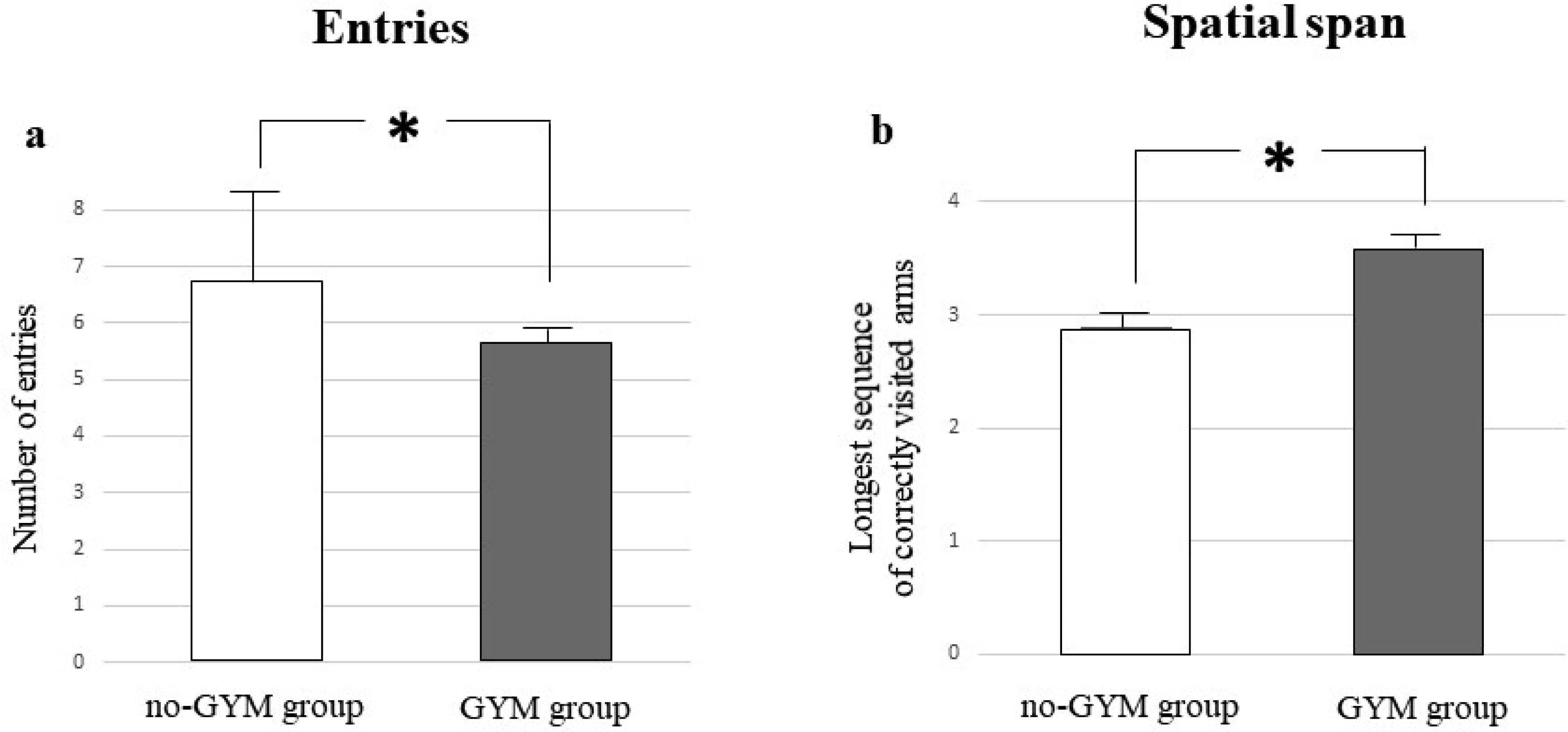
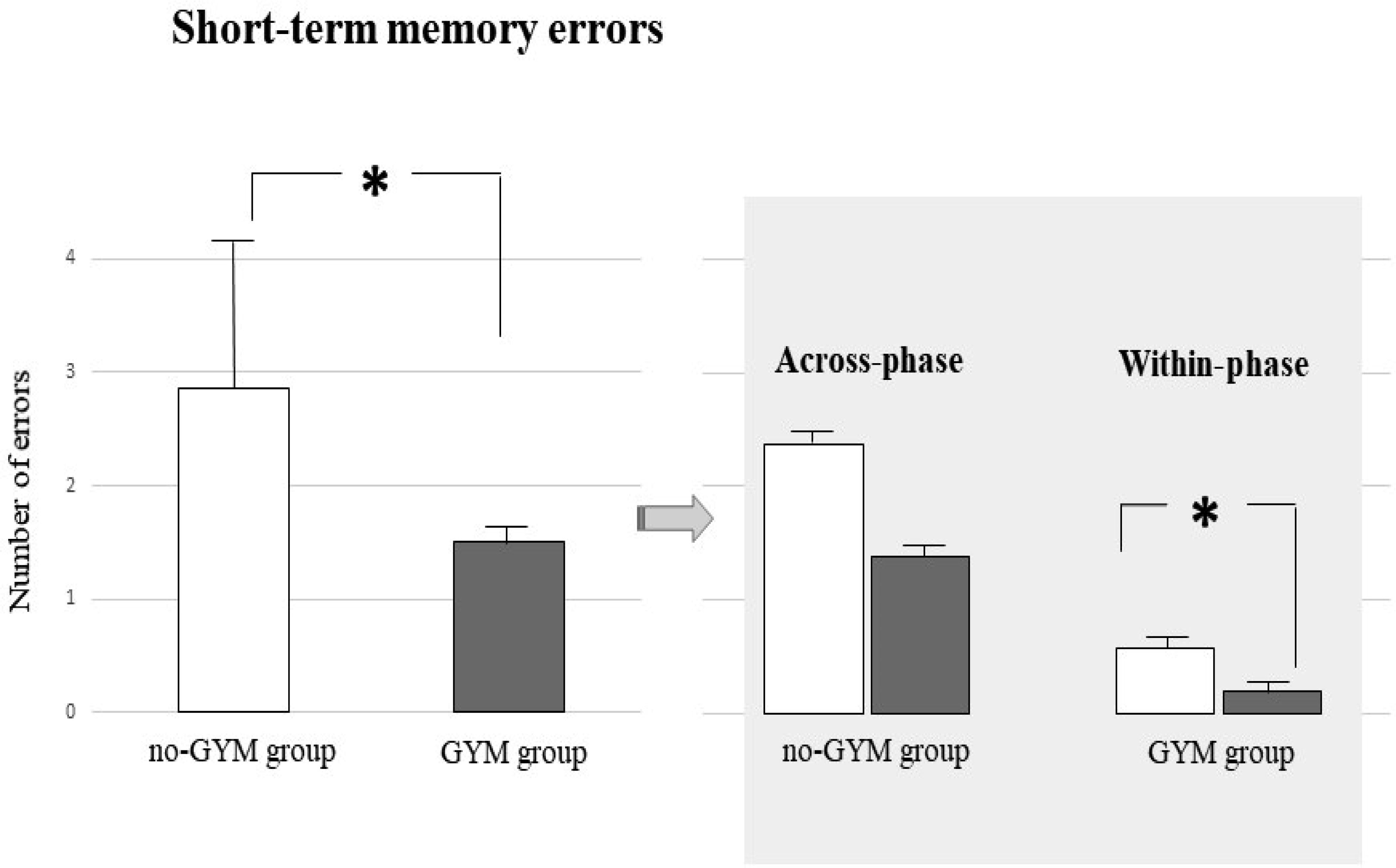
The relationship between physical exercise and improvement in specific cognitive domains in children and adolescents who play sport has been recently reported, although the effects on visuospatial abilities have not yet been well explored. This study is aimed at evaluating in school-age children practicing artistic gymnastics the visuospatial memory by using a table version of the Radial Arm Maze (table-RAM) and comparing their performances with those ones who do not play any sport. The visuospatial performances of 14 preadolescent girls practicing artistic gymnastics aged between 7 and 10 years and those of 14 preadolescent girls not playing any sport were evaluated in the table-RAM forced-choice paradigm that allows disentangling short-term memory from working memory abilities. Data showed that the gymnasts obtained better performances than control group mainly in the parameters evaluating working memory abilities, such as within-phase errors and spatial span. Our findings emphasizing the role of physical activity on cognitive performances impel to promote physical exercise in educational and recreational contexts as well as to analyse the impact of other sports besides gymnastics on cognitive functioning.

Abbreviations

GYM

Gymnastics

Physical Exercise

RAM

Radial Arm Maze

Acknowledgments

This research was partially supported by Italian Ministry of Health (“Linea di Ricerca Corrente A Neurologia Clinica e Comportamentale”, Fondazione Santa Lucia, IRCCS).

Conflict of interest

The authors declare no conflict of interest.

References

[1]	Nithianantharajah J, Hannan AJ (2006) Enriched environments, experience-dependent plasticity and disorders of the nervous system. Nat Rev Neurosci 7: 697-709. doi: 10.1038/nrn1970
[2]	Van der Borght K, Havekes R, Bos T, et al. (2007) Exercise improves memory acquisition and retrieval in the Y-maze task: relationship with hippocampal neurogenesis. Behav Neurosci 121: 324-334. doi: 10.1037/0735-7044.121.2.324
[3]	Ben-Zeev T, Hirsh T, Weiss I, et al. (2020) The Effects of High-intensity Functional Training (HIFT) on Spatial Learning, Visual Pattern Separation and Attention Span in Adolescents. Front Behav Neurosci 14: 577390. doi: 10.3389/fnbeh.2020.577390
[4]	Fernandes J, Arida RM, Gomez-Pinilla F (2017) Physical exercise as an epigenetic modulator of brain plasticity and cognition. Neurosci Biobehav Rev 80: 443-456. doi: 10.1016/j.neubiorev.2017.06.012
[5]	Mandolesi L, Polverino A, Montuori S, et al. (2018) Effects of Physical Exercise on Cognitive Functioning and Wellbeing: Biological and Psychological Benefits. Front Psychol 9: 509. doi: 10.3389/fpsyg.2018.00509
[6]	Biddle SJH, Ciaccioni S, Thomas G, et al. (2019) Physical activity and mental health in children and adolescents: An updated review of reviews and an analysis of causality. Psychol Sport Exerc 42: 146-155. doi: 10.1016/j.psychsport.2018.08.011
[7]	Mandolesi L, Gelfo F, Serra L, et al. (2017) Environmental Factors Promoting Neural Plasticity: Insights from Animal and Human Studies. Neural Plast 2017: 7219461. doi: 10.1155/2017/7219461
[8]	Crawford LK, Caplan JB, Loprinzi PD (2021) The Impact of Acute Exercise Timing on Memory Interference. Percept Mot Skills 128: 1215-1234. doi: 10.1177/0031512521993706
[9]	Lambourne K, Tomporowski P (2010) The effect of exercise-induced arousal on cognitive task performance: a meta-regression analysis. Brain Res 1341: 12-24. doi: 10.1016/j.brainres.2010.03.091
[10]	McMorris T, Hale BJ (2012) Differential effects of differing intensities of acute exercise on speed and accuracy of cognition: a meta-analytical investigation. Brain Cogn 80: 338-351. doi: 10.1016/j.bandc.2012.09.001
[11]	Loprinzi PD, Day S, Hendry R, et al. (2021) The Effects of Acute Exercise on Short- and Long-Term Memory: Considerations for the Timing of Exercise and Phases of Memory. Eur J Psychol 17: 85-103. doi: 10.5964/ejop.2955
[12]	Lees C, Hopkins J (2013) Peer reviewed: effect of aerobic exercise on cognition, academic achievement, and psychosocial function in children: a systematic review of randomized control trials. Prev Chronic Dis 10: E174. doi: 10.5888/pcd10.130010
[13]	Donnelly JE, Hillman CH, Castelli D, et al. (2016) Physical activity, fitness, cognitive function, and academic achievement in children: a systematic review. Med Sci Sports Exerc 48: 1197-1222. doi: 10.1249/MSS.0000000000000901
[14]	Chaddock L, Erickson KI, Prakash RS, et al. (2010) A neuroimaging investigation of the association between aerobic fitness, hippocampal volume, and memory performance in preadolescent children. Brain Res 1358: 172-183. doi: 10.1016/j.brainres.2010.08.049
[15]	Lundbye-Jensen J, Skriver K, Nielsen JB, et al. (2017) Acute exercise improves motor memory consolidation in preadolescent children. Front Hum Neurosci 11: 182. doi: 10.3389/fnhum.2017.00182
[16]	Esteban-Cornejo I, Cadenas-Sanchez C, Contreras-Rodriguez O, et al. (2017) A whole brain volumetric approach in overweight/obese children: Examining the association with different physical fitness components and academic performance. The ActiveBrains project. Neuroimage 159: 346-354. doi: 10.1016/j.neuroimage.2017.08.011
[17]	Hillman CH, Castelli DM, Buck SM (2005) Aerobic fitness and neurocognitive function in healthy preadolescent children. Med Sci Sports Exerc 37: 1967-1974. doi: 10.1249/01.mss.0000176680.79702.ce
[18]	Castelli DM, Hillman CH, Buck SM, et al. (2007) Physical fitness and academic achievement in third-and fifth-grade students. J Sport Exerc Psychol 29: 239-252. doi: 10.1123/jsep.29.2.239
[19]	Verburgh L, Königs M, Scherder EJA, et al. (2014) Physical exercise and executive functions in preadolescent children, adolescents and young adults: a meta-analysis. Br J Sports Med 48: 973-979. doi: 10.1136/bjsports-2012-091441
[20]	Ludyga S, Gerber M, Brand S, et al. (2016) Acute effects of moderate aerobic exercise on specific aspects of executive function in different age and fitness groups: A meta-analysis. Psychophysiology 53: 1611-1626. doi: 10.1111/psyp.12736
[21]	Lott MA, Jensen CD (2017) Executive control mediates the association between aerobic fitness and emotion regulation in preadolescent children. J Pediatr Psychol 42: 162-173.
[22]	Chaddock L, Pontifex MB, Hillman CH, et al. (2011) A review of the relation of aerobic fitness and physical activity to brain structure and function in children. J Int Neuropsychol Soc 17: 975-985. doi: 10.1017/S1355617711000567
[23]	Barker LA (2016) Working memory in the classroom: An inside look at the central executive. Appl Neuropsychol Child 5: 180-193. doi: 10.1080/21622965.2016.1167493
[24]	Cho SY, So WY, Roh HT (2017) The effects of taekwondo training on peripheral neuroplasticity-related growth factors, cerebral blood flow velocity, and cognitive functions in healthy children: A randomized controlled trial. Int J Environ Res Public Health 14: 454. doi: 10.3390/ijerph14050454
[25]	Di Corrado D, Guarnera M, Guerrera CS, et al. (2020) Mental Imagery Skills in Competitive Young Athletes and Non-athletes. Front Psychol 11: 633. doi: 10.3389/fpsyg.2020.00633
[26]	Bidzan-Bluma I, Lipowska M (2018) Physical Activity and Cognitive Functioning of Children: A Systematic Review. Int J Environ Res Public Health 15: 800. doi: 10.3390/ijerph15040800
[27]	O'Keefe J, Nadel L (1978) The hippocampus as a cognitive map Oxford: Oxford University Press, 1-570.
[28]	Stupien G, Florian C, Roullet P (2003) Involvement of the hippocampal CA3- region in acquisition and in memory consolidation of spatial but not in object information in mice. Neurobiol Learn Mem 80: 32-41. doi: 10.1016/S1074-7427(03)00022-4
[29]	Foti F, Sorrentino P, Menghini D, et al. (2020) Peripersonal Visuospatial Abilities in Williams Syndrome Analyzed by a Table Radial Arm Maze Task. Front Hum Neurosci 14: 254. doi: 10.3389/fnhum.2020.00254
[30]	Mandolesi L, Petrosini L, Menghini D, et al. (2009) Children's radial arm maze performance as a function of age and sex. Int J Dev Neurosci 27: 789-797. doi: 10.1016/j.ijdevneu.2009.08.010
[31]	Mandolesi L, Addona F, Foti F, et al. (2009) Spatial competences in Williams syndrome: a radial arm maze study. Int J Dev Neurosci 27: 205-213. doi: 10.1016/j.ijdevneu.2009.01.004
[32]	Jarrard LE, et al. (1993) On the role of hippocampus in learning and memory in the rat. Behav Neural Biol 60: 9-26. doi: 10.1016/0163-1047(93)90664-4
[33]	Mandolesi L, Leggio MG, Spirito F, et al. (2003) Cerebellar contribution to spatial event processing: do spatial procedures contribute to formation of spatial declarative knowledge? Eur J Neurosci 18: 2618-2626. doi: 10.1046/j.1460-9568.2003.02990.x
[34]	Sorrentino P, Lardone A, Pesoli M, et al. (2019) The Development of Spatial Memory Analyzed by Means of Ecological Walking Task. Front Psychol 10: 728. doi: 10.3389/fpsyg.2019.00728
[35]	Overman WH, Pate BJ, Moore K, et al. (1996) Ontogeny of place learning in children as measured in the radial arm maze, Morris search task, and open field task. Behav Neurosci 110: 1205-1228. doi: 10.1037/0735-7044.110.6.1205
[36]	Marina M, Rodríguez FA (2014) Physiological demands of young women's competitive gymnastic routines. Biol Sport 31: 217-222. doi: 10.5604/20831862.1111849
[37]	Erickson KI, Weinstein AM, Sutton BP (2012) Beyond vascularization: aerobic fitness is associated with N-acetylaspartate and working memory. Brain Behav 2: 32-41. doi: 10.1002/brb3.30
[38]	Tressoldi PE, Vio C, Gugliotta M, et al. (2005) BVN 5–11—Batteria per la Valutazione Neuropsicologica per l'età evolutiva Trento: Erickson.
[39]	Xue Y, Yang Y, Huang T (2019) Effects of chronic exercise interventions on executive function among children and adolescents: a systematic review with meta-analysis. Br J Sports Med 53: 1397-1404. doi: 10.1136/bjsports-2018-099825
[40]	de Greeff JW, Bosker RJ, Oosterlaan J, et al. (2018) Effects of physical activity on executive functions, attention and academic performance in preadolescent children: a meta-analysis. J Sci Med Sport 21: 501-507. doi: 10.1016/j.jsams.2017.09.595
[41]	Huang R, Lu M, Song Z, et al. (2015) Long-term intensive training induced brain structural changes in world class gymnasts. Brain Struct Funct 220: 625-644. doi: 10.1007/s00429-013-0677-5
[42]	Fukuo M, Kamagata K, Kuramochi M, et al. (2020) Regional brain gray matter volume in world-class artistic gymnasts. J Physiol Sci 70: 43. doi: 10.1186/s12576-020-00767-w
[43]	Chaddock-Heyman L, Hillman CH, Cohen NJ, et al. (2014) III. The importance of physical activity and aerobic fitness for cognitive control and memory in children. Monogr Soc Res Child Dev 79: 25-50. doi: 10.1111/mono.12129
[44]	Mkaouer B, Hammoudi-Nassib S, Amara S, et al. (2018) Evaluating the physical and basic gymnastics skills assessment for talent identification in men's artistic gymnastics proposed by the International Gymnastics Federation. Biol Sport 35: 383-392. doi: 10.5114/biolsport.2018.78059
[45]	Nardello F, Bertucco M, Cesari P (2021) Anticipatory and pre-planned actions: A comparison between young soccer players and swimmers. PLoS One 16: e0249635. doi: 10.1371/journal.pone.0249635
[46]	Lehnung M, Leplow B, Friege L, et al. (1998) Development of spatial memory and spatial orientation in preschoolers and primary school children. Br J Psychol 89: 463-480. doi: 10.1111/j.2044-8295.1998.tb02697.x
[47]	Passolunghi MC, Mammarella IC (2012) Selective spatial working memory impairment in a group of children with mathematics learning disabilities and poor problem-solving skills. J Learn Disabil 45: 341-350. doi: 10.1177/0022219411400746

Reader Comments

Your name:*

Email:*
© 2021 the Author(s), licensee AIMS Press. This is an open access article distributed under the terms of the Creative Commons Attribution License (http://creativecommons.org/licenses/by/4.0)