An investor uses the graphical presentation of Bollinger Bands to get signals of the ups and downs, as well the volatility of the market from the expansion and tightening of the UBB and LBB, reflecting higher and lower volatility. The percent (%) b helps determine the opportunities during extreme periods from the market, looking at the concentration of line graph at the value "0" or "1" reflecting the bearish and bullish trend, respectively. The Bandwidth Index was able to picture out the bullish trend with a squeeze at the upper band. The positive unimodality of Q for NEPSE daily return for the period of the fiscal year 1998–1999 to the fiscal year 2019–2020 indicated normality for the market return. Nevertheless, the results for the trading signals based on the Bollinger bands are seen as useful for an investor by giving a clear signal to "buy" or "sell". At the same time, relying only on Bollinger Bands with a specific period MA, i.e. the Bollinger Bands with a shorter moving average (MA) shows higher fluctuations and vice-versa, hence, could show false signals while choosing inappropriate MA, therefore, help of other technical analysis tools should be taken while going for an investment decision.
Citation: Rashesh Vaidya. NEPSE in Bollinger Bands[J]. National Accounting Review, 2021, 3(4): 439-451. doi: 10.3934/NAR.2021023
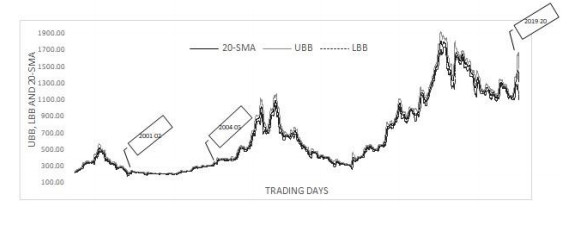
An investor uses the graphical presentation of Bollinger Bands to get signals of the ups and downs, as well the volatility of the market from the expansion and tightening of the UBB and LBB, reflecting higher and lower volatility. The percent (%) b helps determine the opportunities during extreme periods from the market, looking at the concentration of line graph at the value "0" or "1" reflecting the bearish and bullish trend, respectively. The Bandwidth Index was able to picture out the bullish trend with a squeeze at the upper band. The positive unimodality of Q for NEPSE daily return for the period of the fiscal year 1998–1999 to the fiscal year 2019–2020 indicated normality for the market return. Nevertheless, the results for the trading signals based on the Bollinger bands are seen as useful for an investor by giving a clear signal to "buy" or "sell". At the same time, relying only on Bollinger Bands with a specific period MA, i.e. the Bollinger Bands with a shorter moving average (MA) shows higher fluctuations and vice-versa, hence, could show false signals while choosing inappropriate MA, therefore, help of other technical analysis tools should be taken while going for an investment decision.

| [1] | Baiynd AM (2011) The Trading Book: A Complete Solution to Mastering Technical Systems and Trading Psychology, New York: McGraw Hill. |
| [2] | Balsara NJ, Chen G, Zheng L (2007) The Chinese stock market: An examination of the random walk model and technical trading rules. Qtly J Bus Eco 46: 43–63. |
| [3] | Bollinger J (1992) Using Bollinge Bands. Techn Anal Stks Commit 10: 47–51. |
| [4] | Bollinger J (2001) Bollinger on Bollinger Bands, New York: McGraw Hill Education. |
| [5] | Chandima AVL (2021) Use stock market data to assist investors on getting more accurate transaction decision. Intl J Sci Res Pub 11: 762–770. |
| [6] | Chen SL, Chen NJ, Chuang RJ (2014) An empirical study on technical analysis: GARCH (1, 1) model. J Appl Stat 41: 785–801. |
| [7] | Chen S, Zhang B, Zhou G, et al. (2018) Bollinger Bands trading strategy based on wavelet analysis. Appl Econ Financ 5: 49–58. |
| [8] | Evans HP (2008) An empirical study of rotational trading using the %b oscillator. J Techn Anal 65: 35–41. |
| [9] | Fang J, Jacobsen B, Qin Y (2014) Popularity versus profitability: Evidence from Bollinger Bands. SSRN Electro J, 1–45. |
| [10] | Ibrahim D (2013) Etude théorique d'indicateurs d'analyse technique [Theoretical Study of Technical Analysis Indicators].Université Nice Sophia Antipolis, Finance Quantitative Français: HAL archives-ouvertes. |
| [11] | Kabasinskas A, Macys U (2010) Calibration of Bollinger Bands parameters for trading strategy development in the Baltic stock market. Inzinerine Ekonomika-Eng Econ 21: 244–254. |
| [12] | Kannan KS, Sekar PS, Sathik MM, et al. (2010) Financial Stock Market Forecast using Data Mining Techniques. Proceedings of the Intl Multi Conf of Eng and Computer Scientists (IMECS), I, March 17–19, 1–5. |
| [13] | Khairi TWA, Zaki RM, Mahmood WA (2019) Stock price prediction using technical, fundamental and news based approach. 2nd Sc. Conf of Computer Sci (SCCS), March 27–28,171–181. |
| [14] | Kirkpatrick CD, Dahlquist JR (2015) Technical Analysis: The Complete Resource for Financial Market Technicians, New Jersy: Pearson Education, Inc. |
| [15] | Lee J, Lee J, Prxekopa A (2013) Price-Bands: A Technical Tool for Stock Trading, New Jersy: Rutgers University. |
| [16] | Lento C, Gradojevic N (2007) The profitability of trading rules: A combined signal approach. J Appl Bus Res 23: 13–28. |
| [17] | Lento C, Gradojevic N, Wright CS (2007) Investment information content in Bollinger Bands? Appl Financ Econ Lets 3: 263–267. |
| [18] | Leung JM, Chong TT (2003) An empirical comparison of moving average envelops and Bollinger Bands. Appl Econ Lets 10: 339–341. |
| [19] | Lim S, Hisarli TT, Shi He N (2014) The profitability of a combined signal approach: Bollinger Bands and the ADX. Intl Fed Techn Anal J (IFTA Journal) 14: 30–36. |
| [20] | Liu W, Huang X, Zheng W (2006) Black-Scholes' model and Bollinger Bands. Phys A 371: 565–571. |
| [21] | Mkik M, Menzhi K (2020) The profitability of chartist analysis: Case of the Bollinge Bands indicator. IOSR J Econ Financ 11: 30–34. |
| [22] | Ni Y, Day MY, Huang P, et al. (2020) The profitability of Bollinger Bands: Evidence from the constituent stocks of Taiwan. Phys A 551: 124144. |
| [23] | Pramudya R, Ichsani S (2020) Efficiency of technical analysis for stock trading. Intl J Financ Bank Stud 9: 58–67. |
| [24] | Prasad TD, Chaitanya C, Kumar AT (2018) A study on stock's volatility in banking sector using technical analysis. Intl Res J Eng Tech 05: 1016–1022. |
| [25] | Pushpa BV, Sumithra CG, Hegde M (2017) Investment decision making using technical analysis: A study on select stocks in Indian stock market. IOSR J Econ Financ 19: 24–33. |
| [26] | Rachev ST, Menn C, Fabozzi FJ (2005) Fat Tailed and Skewed Asset Return Distributions, Implications for Risk Management, Portfolio Selection, and Option Pricing, New York: John Wiley. |
| [27] | Shah NP, Patel TM (2015) A comparative study on technical analysis by Bollinger Band and RSI. Intl J Mgmt Soci Sci 03: 234–251. |
| [28] | Singh A, Gupta P, Thakur N (2021) An emprical research and comprehensive analysis of stock market prediction using machine learning and deep learning techniques. Intl Conf Comput Res and Data Analyt (ICCRDA 2020), IOP Conf Ser.: Mater. Sci. Eng., 10220(12098), October 24, 1–13. |
| [29] | Williams B (2013) Volatility-Based Support Trading. Futures: News, Analysis & Strategies for Futures. Opts Derivs Traders 42: 20–22. |
| [30] | Williams OD (2006) Emprical Optimization of Bollinger Bands for Profitability, Bumaby: Simon Fraser Univeristy. |


Figures(4) / Tables(1)

Rashesh Vaidya. NEPSE in Bollinger Bands[J]. National Accounting Review, 2021, 3(4): 439-451. doi: 10.3934/NAR.2021023


 DownLoad: