
Citation: Zhenshu Wen, Lijuan Shi. Exact explicit nonlinear wave solutions to a modified cKdV equation[J]. AIMS Mathematics, 2020, 5(5): 4917-4930. doi: 10.3934/math.2020314
[1] | Chen Peng, Zhao Li . Optical soliton solutions for Lakshmanan-Porsezian-Daniel equation with parabolic law nonlinearity by trial function method. AIMS Mathematics, 2023, 8(2): 2648-2658. doi: 10.3934/math.2023138 |
[2] | M. A. El-Shorbagy, Sonia Akram, Mati ur Rahman, Hossam A. Nabwey . Analysis of bifurcation, chaotic structures, lump and $ M-W $-shape soliton solutions to $ (2+1) $ complex modified Korteweg-de-Vries system. AIMS Mathematics, 2024, 9(6): 16116-16145. doi: 10.3934/math.2024780 |
[3] | Feiting Fan, Xingwu Chen . Dynamical behavior of traveling waves in a generalized VP-mVP equation with non-homogeneous power law nonlinearity. AIMS Mathematics, 2023, 8(8): 17514-17538. doi: 10.3934/math.2023895 |
[4] | Harivan R. Nabi, Hajar F. Ismael, Nehad Ali Shah, Wajaree Weera . W-shaped soliton solutions to the modified Zakharov-Kuznetsov equation of ion-acoustic waves in (3+1)-dimensions arise in a magnetized plasma. AIMS Mathematics, 2023, 8(2): 4467-4486. doi: 10.3934/math.2023222 |
[5] | A. K. M. Kazi Sazzad Hossain, M. Ali Akbar . Solitary wave solutions of few nonlinear evolution equations. AIMS Mathematics, 2020, 5(2): 1199-1215. doi: 10.3934/math.2020083 |
[6] | Ikram Ullah, Muhammad Bilal, Javed Iqbal, Hasan Bulut, Funda Turk . Single wave solutions of the fractional Landau-Ginzburg-Higgs equation in space-time with accuracy via the beta derivative and mEDAM approach. AIMS Mathematics, 2025, 10(1): 672-693. doi: 10.3934/math.2025030 |
[7] | Khalid Khan, Amir Ali, Muhammad Irfan, Zareen A. Khan . Solitary wave solutions in time-fractional Korteweg-de Vries equations with power law kernel. AIMS Mathematics, 2023, 8(1): 792-814. doi: 10.3934/math.2023039 |
[8] | Mustafa Inc, Hadi Rezazadeh, Javad Vahidi, Mostafa Eslami, Mehmet Ali Akinlar, Muhammad Nasir Ali, Yu-Ming Chu . New solitary wave solutions for the conformable Klein-Gordon equation with quantic nonlinearity. AIMS Mathematics, 2020, 5(6): 6972-6984. doi: 10.3934/math.2020447 |
[9] | F. A. Mohammed, Mohammed K. Elboree . Soliton solutions and periodic solutions for two models arises in mathematical physics. AIMS Mathematics, 2022, 7(3): 4439-4458. doi: 10.3934/math.2022247 |
[10] | Noorah Mshary . Exploration of nonlinear traveling wave phenomena in quintic conformable Benney-Lin equation within a liquid film. AIMS Mathematics, 2024, 9(5): 11051-11075. doi: 10.3934/math.2024542 |
As is well known, the Korteweg-de Vries (KdV) equation has attracted much attention due to its significant nature in physical contexts, stratified internal waves, ion-acoustic wave, plasma physics [1]. Many generalized forms of KdV equation have been introduced, such as modified KdV (mKdV) equation and high-order KdV equation. Besides, There has been considerate studies on time-delayed KdV-related equation. Zhao and Xu [2] dealt with the existence of solitary waves for KdV equation with time delay. Liu et al. [3] studied the KdV-Burgers-Kuramoto chaotic system with distributed delay feedback and analyzed the conditions under which Hopf bifurcation occurs. Baudouin et al. [4] employed two approaches to study the stability of the nonlinear KdV equation with boundary time-delay feedback. Komornik and Pignotti [5] considered well-posedness and exponential decay estimates for a KdV-Burgers equation with time-delay.
In this paper, we focus on the following modified coupled Korteweg-de Vries (cKdV) equation,
{ut=vx−32uux+αux,vt=14uxxx−vux−12uvx+αvx, | (1.1) |
where α is a constant, which was introduced in [6]. As suggested in [6,7,8,9], Eq (1.1) is a general example of N-component systems, energy dependent schrödinger operators and bi-Hamiltonian structures for multi-component systems. The authors in [6] studied the soliton solutions to Eq (1.1), and demonstrated the soliton fission effect, kink to anti-kink transitions, and multipeaked solitons by using a class of commuting Hamiltonian systems on Riemann surfaces. Additionally, they indicated that many important equations that model physical phenomena in fluid dynamics and nonlinear optics, such as the generalized Kaup equation, the classical Boussinesq equation and the systems governing second harmonic generation (SHG), are connected to the cKdV equation through nonsingular transformations [6], which potentially enables solutions of cKdV equations to be interpreted in the context of these related equations. Besides, Wen and Wang [10] constructed some exact explicit solutions to Eq (1.1) by employing the three forms of (ω/g)-expansion method, i.e., (g′/g2)-expansion method, (g′/g)-expansion method and (g′)-expansion method.
In this paper, we further study nonlinear wave solutions to Eq (1.1) from the perspective of dynamical systems [11,12,13,14,15,16,17,18,19,20,21,22,23,24,25,26,27,28]. More preciously, we first transform Eq (1.1) into a planar system, identify all possible bifurcation conditions, and obtain the phase portraits of the system in the different regions of the parametric space. Further, we seek to obtain exact explicit expressions of nonlinear wave solutions to Eq (1.1), including solitary wave solutions, singular wave solutions, periodic singular wave solutions, and kink (antikink) wave solutions. More interestingly, we find the so-called V-shaped kink (antikink) wave solutions, W-shaped solitary wave solutions, and W-shaped periodic wave solutions. To improve the readability of the paper, we give the definitions of these kinds of solutions here. Suppose that φ(ξ) with ξ=x−ct is a traveling wave solution of the equation. Solitary wave solution φ(ξ) means that φ(ξ) satifies limξ→±∞φ(ξ) exist and limξ→+∞φ(ξ)=limξ→−∞φ(ξ). Singular wave solution φ(ξ) means that φ(ξ) blow up at some point, that is, there exists some point ξ0 such that limξ→ξ0φ(ξ)=±∞. Periodic singular wave solution φ(ξ) means that φ(ξ) blow up at some points periodically. Kink (antikink) wave solution φ(ξ) means that φ(ξ) satifies limξ→±∞φ(ξ) exist and limξ→+∞φ(ξ)>limξ→−∞φ(ξ) (limξ→+∞φ(ξ)<limξ→−∞φ(ξ)). V-shaped kink (antikink) wave solution φ(ξ) means that φ(ξ) is a kink (antikink) wave solution with one valley, such as Figure 4(b) (4(c)). W-shaped solitary wave solution φ(ξ) means that φ(ξ) is a solitary wave solution with one hump and two valleys, such as Figure 4(b). W-shaped periodic solitary wave solution φ(ξ) means that φ(ξ) is a W-shaped solitary wave solution and it is periodic, such as Figure 5(b) and 5(d).
The remaining paper is organized as follows. In section 2, we outline the procedure of identifying the bifurcation conditions and obtaining the phase portraits of the corresponding planar system in the different regions of the parametric space. In section 3, we present the main results about exact explicit of nonlinear wave solutions to Eq (1.1), especially, the V-shaped kink (antikink) wave solutions, W-shaped solitary wave solutions, and W-shaped periodic wave solutions, and the proof follows. Section 4 is devoted to numerical simulations of solutions. The paper is ended with the conclusion.
In this section, we identify the bifurcation conditions and derive the phase portraits corresponding to Eq (1.1).
For given constant c, substituting u(x,t)=u(ξ), v(x,t)=v(ξ) with ξ=x−ct into Eq (1.1), it follows,
{cu′+v′−32uu′+αu′=0,cv′+14u‴−vu′−12uv′+αv′=0, | (2.1) |
where the prime stands for the derivative with respect to ξ.
Integrating the first equation of (2.1) once leads to
v=34u2−(c+α)u+g14, | (2.2) |
where g1 is integral constant.
Substituting (2.2) into the second equation of (2.1) and integrating the equation, it follows that
u″−2u3+6(c+α)u2−4(c+α)2u−g1u+g2=0, |
where g2 is integral constant.
Letting y=u′, we obtain a planar system
{dudξ=y,dydξ=2u3−6(c+α)u2+(4(c+α)2+g1)u−g2. | (2.3) |
By setting φ=u−(c+α), system (2.3) becomes
{dφdξ=y,dydξ=2φ3+(g1−2(c+α)2)φ+g1(c+α)−g2, | (2.4) |
with Hamiltonian
H(φ,y)=y22−φ42−12(g1−2(c+α)2)φ2−(g1(c+α)−g2)φ. | (2.5) |
To study the singular points of system (2.5), let
f(φ)=2φ3+(g1−2(c+α)2)φ+g1(c+α)−g2, | (2.6) |
and
f0(φ)=2φ3+(g1−2(c+α)2)φ. | (2.7) |
Obviously, if g1<2(c+α)2, then f0(φ) has three zero points,
φ=0,±φ1, | (2.8) |
where φ1=√12(2(c+α)2−g1). In addition, it is easy to obtain the two extreme points of f(φ) as follows
φ∗±=√16(2(c+α)2−g1). | (2.9) |
Let
g0=|f0(φ∗±)|=√227(2(c+α)2−g1)3, | (2.10) |
which denotes the absolute value of extreme values of f0(φ). Now we can easily give the profiles of f(φ) in Figure 1.
Let (φi,0) be one of the singular points of system (2.4). Then the characteristic values of the linearized system of system (2.4) at the singular point (φi,0) are
λ±=±√f′(φi). | (2.11) |
From Figure 1 and Eq (2.11), we can determine the number of singular points and their dynamical behaviors (saddles, centers, etc.). Furthermore, note that when g2=g1(c+α), we have H(φ1,0)=H(−φ1,0), which indicates that the two saddles (±φ1,0) connect.
Based on the above analysis, we obtain the phase portraits of system (2.4) in Figure 2. Note that in the phase portraits φ2=−2√16(2(c+α)2−g1) and the other φis are given in Section 3.
Remark 1. In the above analysis, we have supposed that g1<2(c+α)2. In fact, when g1≥2(c+α)2, system (2.4) has only one saddle and the phase portrait is similar with Figure 2(a) or 2(g). Therefore, we omit the case when g1≥2(c+α)2.
In this section, we state our results about solitary wave solutions, singular wave solutions, periodic singular wave solutions, and kink (antikink) wave solutions for the component u(x,t) of Eq (1.1), and especially, we emphasize the results of the V-shaped kink (antikink) wave solution, W-shaped solitary wave solution, and W-shaped periodic wave solution for the component v(x,t) of Eq (1.1). Note that the relation between the solutions of Eq (1.1) and the solutions of system (2.4) can be derived through the transformations u(x,t)=u(ξ) and φ(ξ)=u(ξ)−(c+α) with ξ=x−ct. To relate conveniently, we also omit the expression of the component v(x,t) of Eq (1.1), i.e., v(x,t)=34u2(x,t)−(c+α)u(x,t)+g14, in the following theorems.
Theorem 1. When g2=g1(c+α), Eq (1.1) has two kink (antikink) wave solutions
u(x,t)=±φ1tanh(φ1(x−ct))+c+α, | (3.1) |
two singular wave solutions
u(x,t)=±φ1coth(φ1(x−ct))+c+α, | (3.2) |
four periodic singular wave solutions
u(x,t)=±√2φ1csc(√2φ1(x−ct))+c+α, | (3.3) |
u(x,t)=±√2φ1sec(√2φ1(x−ct))+c+α, | (3.4) |
and a family of periodic wave solutions
u(x,t)=−2α1α2sn2((x−ct)/ρ1,κ1)+α1(α1+α2)2α1sn2((x−ct)/ρ1,κ1)−(α1+α2), | (3.5) |
where ρ1=2α1+α2,κ1=2√α1α2α1+α2, ±α1,±α2 are four roots of H(φ,y)=h,h∈(H(0,0),H(φ1,0)). In addition, when h→H(φ1,0), the periodic wave solution (3.5) tends to the kink (antikink) wave solutions (3.1).
Furthermore, if c, α, and g1 satisfy the condition −φ1<−c+α3<φ1, then the component v(x,t)=34u2(x,t)−(c+α)u(x,t)+g14 corresponding to the kink (antikink) wave solutions (3.1) are the V-shaped kink (antikink) wave solutions. In addition, if c, α, g1, and h satisfy the condition −α1<−c+α3<α1, then the component v(x,t)=34u2(x,t)−(c+α)u(x,t)+g14 corresponding to the periodic wave solution (3.5) is the W-shaped periodic wave solution.
Proof. When g2=g1(c+α), we consider the following three types of orbits.
(i) First, there are two heteroclinic orbits Γ±1 connected at two saddle points (φ1,0) and (−φ1,0) from Figure 2(d), which can be expressed, from (2.5),
y=±(φ21−φ2). | (3.6) |
Substituting (3.6) into the first equation of system (2.4), and integrating along the heteroclinic orbits, it follows that
∫φ0dsφ21−s2=|ξ|, | (3.7) |
and
∫+∞φdss2−φ21=|ξ|. | (3.8) |
From (3.7) and (3.8), we get two kink (antikink) wave solutions (3.1) and two singular wave solutions (3.2).
(ii) Second, from Figure 2(d), there are two special orbits Γ±2, which have the same hamiltonian with that of the center point (0,0). In (φ,y)−plane, from (2.5), the expressions of these two orbits Γ±2 are given as
y=±φ√φ2−2φ21. | (3.9) |
Substituting (3.9) into the first equation of system (2.4), and integrating along the two orbits Γ±2, it follows that
∫+∞φdss√s2−2φ21=|ξ|. | (3.10) |
From (3.10), we get two periodic singular wave solutions (3.3).
Further, note that if φ=φ(ξ) is a solution of system, then φ=φ(ξ+γ) is also a solution of system. Specially, we take γ=π2, we obtain another two periodic singular solutions (3.4).
(iii) Third, from Figure 2(d) or more specifically Figure 3(a), there exist one family of periodic orbits defined by H(φ,y)=h,h∈(H(0,0),H(φ1,0)), the expressions of which are given by
y=±√(α22−φ2)(α21−φ2). | (3.11) |
Substituting (3.11) into the first equation of system (2.4), and integrating along the families of periodic orbits, it follows that
∫φ−α11√(α22−s2)(α21−s2)ds=|ξ|. | (3.12) |
From (3.12), we derive the family of periodic wave solutions (3.5) by the elliptic integral [29].
The convergence result follows from α1→φ1, when h→H(φ1,0).
Furthermore, if c, α, and g1 satisfy the condition −φ1<−c+α3<φ1, then we have −φ1+c+α3<0<φ1+c+α3. Note that the component u(x,t) in (3.1) satisfies u(x,t)∈(−φ1+c+α,φ1+c+α). It follows from the expression v(x,t)=34u2(x,t)−(c+α)u(x,t)+g14=34(u(x,t)−23(c+α))2+g14−13(c+α)2 that the component v(x,t) corresponding to (3.1) is the V-shaped kink (antikink) wave solutions, the profiles of which are shown in Figure 4(b) and 4(c). In addition, if c, α, g1, and h satisfy the condition −α1<−c+α3<α1, then one has −α1+c+α3<0<α1+c+α3. Note that the component u(x,t) in (3.5) satisfies u(x,t)∈(−α1+c+α,α1+c+α). It follows from the expression v(x,t)=34u2(x,t)−(c+α)u(x,t)+g14=34(u(x,t)−23(c+α))2+g14−13(c+α)2 that the component v(x,t) corresponding to (3.5) is the W-shaped periodic wave solution, the profile of which is shown in Figure 5(b).
Theorem 2. When g1(c+α)−g0<g2<g1(c+α), Eq (1.1) has one solitary wave solution
u(x,t)=φ6−2θ1(φ61−φ62)cosh(√θ1(x−ct))+4φ6+c+α, | (3.13) |
one singular wave solution
u(x,t)=φ6+θ12φ6cosh(√θ1(x−ct))−√θ1sinh(√θ(x−ct))−2φ6+c+α, | (3.14) |
where θ1=(φ6−φ61)(φ6−φ62), one periodic singular wave solution
u(x,t)=φ5−2θ2(φ51−φ52)sin(arcsin(4φ5φ51−φ52)−√θ2(x−ct))−4φ5+c+α, | (3.15) |
where θ2=(φ51−φ5)(φ5−φ52), and a family of periodic wave solutions
u(x,t)=α3(α5−α4)sn2((x−ct)/ρ2,κ2)−α4(α5−α3)(α5−α4)sn2((x−ct)/ρ2,κ2)−(α5−α3), | (3.16) |
where ρ2=2√(α6−α4)(α5−α3),κ2=√(α5−α4)(α6−α3)(α6−α4)(α5−α3) and α3,α4,α5,α6 are four roots of H(φ,y)=h,h∈(H(φ5,0),H(φ6,0)). In addition, when h→H(φ6,0), the periodic wave solution (3.16) tends to the solitary wave solution (3.13).
Furthermore, if c, α, g1, and g2 satisfy the condition φ61<−c+α3<φ6, then the component v(x,t)=34u2(x,t)−(c+α)u(x,t)+g14 corresponding to (3.13) is the W-shaped solitary wave solution. In addition, if c, α, g1, g2 and h satisfy the condition α4<−c+α3<α5, then the component v(x,t)=34u2(x,t)−(c+α)u(x,t)+g14 corresponding to (3.16) is the W-shaped periodic wave solution.
Proof. When g1(c+α)−g0<g2<g1(c+α), denote the maximum zero of f(φ) as
φ6=√λ6(2(c+α)2−g1), |
where λ is a parameter with 1<λ<3, then we can obtain the other two zeros of f(φ)
φ4=−12√λ6(2(c+α)2−g1)(√12λ−3+1),φ5=12√λ6(2(c+α)2−g1)(√12λ−3−1), |
we have,
(i) First, there is a homoclinic orbit Γ3, which passes the saddle point (φ6,0) in Figure 2(c). In (φ,y)−plane, from (2.5), the expressions of the homoclinic orbit are given as
y=±√(φ6−φ)2(φ−φ61)(φ−φ62), φ62<φ61<φ<φ6. | (3.17) |
Substituting (3.17) into the first equation of system (2.4), and integrating along the homoclinic orbit, it follows that
∫φφ61ds(φ6−s)√(s−φ61)(s−φ62)=|ξ|, | (3.18) |
and
∫+∞φds(s−φ6)√(s−φ61)(s−φ62)=|ξ|. | (3.19) |
From (3.18) and (3.19), we get the solitary wave solutions (3.13) and the singular wave solution (3.14).
(ii) Second, from Figure 2(c), there are another two special orbits Γ±4, which have the same hamiltonian with that of the center point (φ5,0). In (φ,y)−plane, from (2.5), the expressions of these two orbits Γ±4 are given as
y=±√(φ−φ5)2(φ−φ51)(φ−φ52), φ52<φ5<φ51, | (3.20) |
where
φ51=√λ6(2(c+α)2−g1)(√√λ12−3+1−12(√12λ−3−1)), |
and
φ52=−√λ6(2(c+α)2−g1)(√√λ12−3+1+12(√12λ−3−1)). |
Substituting (3.20) into the first equation of system (2.4), and integrating along these two special orbits Γ±4, it follows that
∫+∞φds(s−φ5)√(s−φ51)(s−φ52)=|ξ|. | (3.21) |
From (3.21), we get the periodic singular wave solution (3.15).
(iii) Third, from Figure 2(c) or more specifically Figure 3(b), there exist one family of periodic orbits defined by H(φ,y)=h,h∈(H(φ5,0),H(φ6,0)), the expressions of which are given by
y=±√(α6−φ)(α5−φ)(φ−α4)(φ−α3), α4<φ<α5. | (3.22) |
Substituting (3.22) into the first equation of (2.4) and integrating along the family of periodic orbits, it follows that
∫φα41√(α6−s)(α5−s)(s−α4)(s−α3)ds=|ξ|. | (3.23) |
From (3.23), we derive the family of periodic wave solutions (3.16) by the elliptic integral formula 254.00 in [29].
The convergence result follows from α3→φ62, α4→φ61, α5→φ6, and α6→φ6, when h→H(φ6,0).
Furthermore, if c, α, g1, and g2 satisfy the condition φ61<−c+α3<φ6, then we have φ61+c+α3<0<φ6+c+α3. Note that the component u(x,t) in (3.13) satisfies u(x,t)∈(φ61+c+α,φ6+c+α). It follows from the expression v(x,t)=34u2(x,t)−(c+α)u(x,t)+g14=34(u(x,t)−23(c+α))2+g14−13(c+α)2 that the component v(x,t) corresponding to (3.13) is the W-shaped solitary wave solution, the profile of which is shown in Figure 6(b). Similarly, if c, α, g1, g2, and h satisfy the condition α4<−c+α3<α5, then we have α4+c+α3<0<α5+c+α3. Note that the component u(x,t) in (3.16) satisfies u(x,t)∈(α4+c+α,α5+c+α). It follows from the expression v(x,t)=34u2(x,t)−(c+α)u(x,t)+g14=34(u(x,t)−23(c+α))2+g14−13(c+α)2 that the component v(x,t) corresponding to (3.16) is the W-shaped periodic wave solution, the profile of which is shown in Figure 5(d).
Theorem 3. When g2=g1(c+α)−g0, Eq (1.1) has two singular wave solutions
u(x,t)=φ3(−3−(2φ3(x−ct)+1)2)1−(2φ3(x−ct)+1)2+c+α, | (3.24) |
and
u(x,t)=φ3(−3−4(φ3)2(x−ct)2)1−4(φ3)2(x−ct)2+c+α, | (3.25) |
where φ3=√16(2(c+α)2−g1).
Proof. When g2=g1(c+α)−g0, from Figure 2(b), there are two orbits Γ±5, which have the same hamiltonian with the degenerate saddle point (φ3,0). In (φ,y)−plane, from (2.5), the expressions of these two orbits Γ±5 are given as
y=±√(φ−φ3)3(φ−φ31), | (3.26) |
where φ31=−3√16(2(c+α)2−g1).
Substituting (3.26) into the first equation of system (2.4), and integrating along these two orbits Γ±5, it follows that
∫+∞φds(s−φ3)√(s−φ3)(s−φ31)=|ξ|, | (3.27) |
and
∫φ31φds(φ3−s)√(φ3−s)(φ31−s)=|ξ|. | (3.28) |
From (3.27) and (3.28), we get two singular wave solutions (3.24) and (3.25).
Remark 2. In general, the homoclinic orbit corresponds to the solitary wave solution, the heteroclinic orbit corresponds to the kink (antikink) wave solution, the periodic orbit corresponds to the periodic wave solution and the unbounded orbit corresponds to the singular wave solution.
Taking α=3,c=4,g1=2,g2=14,h=1152, which indicates that g2=g1(c+α),−φ1=−4√3<c+α3=73<φ1=4√3,h=H(φ1), we illustrate the profiles of the kink (antikink) wave solutions u(x,t) in (3.1) and the corresponding v(x,t) in Figure 4(a), 4(b) and 4(c). Interestingly, the solutions v(x,t) corresponding to the kink (antikink) wave solutions u(x,t) in (3.1) are the V-shaped kink (antikink) wave solutions. In addition, If we take α=3,c=4,g1=2,g2=14,h=1100, then g2=g1(c+α),−α1=−6.148<c+α3=73<α1=6.148,h∈(H(0,0),H(φ1,0))=(0,1152), and we illustrate the profiles of the periodic wave solutions u(x,t) in (3.5) and the corresponding v(x,t) in Figure 5(a) and 5(b). Now we find that the solution v(x,t) corresponding to the periodic wave solution u(x,t) in (3.5) is the W-shaped periodic wave solution.
Similarly, we choose α=3,c=4,g1=2,g2=3,h=1176.11, such that g1(c+α)−g0<g2<g1(c+α), φ61=−5.6<c+α3=73<φ=6.87,λ=2.95∈(1,3),h=H(φ6). Under these parameter conditions, the profiles of the solitary wave solution u(x,t) in (3.13) and the corresponding v(x,t) are shown in Figure 6(a) and 6(b). The solution v(x,t) corresponding to the solitary wave solution u(x,t) in (3.13) is the W-shaped solitary wave solution. Additionally, if choosing α=3,c=4,g1=2,g2=3,h=1000, then g1(c+α)−g0<g2<g1(c+α),α4= −5.246<c+α3=73<α5=5.9, λ=2.95∈(1,3),h∈(H(φ5,0),H(φ6,0))=(−0.63,1176.11), and we illustrate the profiles of the periodic wave solution u(x,t) in (3.16) and the corresponding v(x,t) in Figure 5(c) and 5(d). Now the solution v(x,t) corresponding to the periodic wave solution u(x,t) in (3.16) is the W-shaped periodic wave solution.
Remark 3. In the above theorems, we just list the results when g2≤g1(c+α), since the results when g2>g1(c+α) can be derived similarly. Here, we deduce that the profiles of the solutions when g2>g1(c+α) will be completely symmetric to the corresponding profiles of the solutions when g2<g1(c+α) about the ξ-axis.
In this paper, by employing the bifurcation method and qualitative theory of dynamical systems, we study the nonlinear wave solutions to the modified cKdV equation (1.1), and obtain exact explicit expressions of the various types of nonlinear wave solutions, including solitary wave solutions, singular wave solutions, periodic singular wave solutions, and kink (antikink) wave solutions. Among these solutions, of particular interest is the appearance of the so-called V-shaped kink (antikink) wave solutions, W-shaped solitary wave solutions, and W-shaped periodic wave solutions, which were not found previously. These solutions may be interpreted in the context of some related equations, such as the generalized Kaup equation, the classical Boussinesq equation and the systems governing second harmonic generation (SHG), which are connected to the cKdV equation (1.1) through nonsingular transformations [6]. Additionally, in the Theorems 1 and 2, we see that if the parameters c,α,g1 and g2 satisfies certain conditions, the V-shaped kink (antikink) wave solutions, W-shaped solitary wave solutions, and W-shaped periodic wave solutions are found. This potentially provide a way to control the appearance of these interesting solutions. Finally, we know that time delay and perturbation play an important in modeling mathematics physics problems [30], so we may further study the solutions and their properties of the time delayed or perturbed version of Eq (1.1).
This research is partially supported by the National Natural Science Foundation of China (No. 11701191), the Fundamental Research Funds for the Central Universities (No. ZQN-802), Program for Innovative Research Team in Science and Technology in Fujian Province University, and Quanzhou High-Level Talents Support Plan under Grant 2017ZT012.
All authors declare no conflicts of interest in this paper.
[1] | M. J. Ablowitz, P. A. Clarkson, Solitons, Nonlinear Evolution Equations and Inverse Scattering, London Math. Soc., London, 1991. |
[2] | Z. Zhao, Y. Xu, Solitary waves for Korteweg-de Vries equation with small delay, J. Math. Anal. Appl., 368 (2010), 43-53. |
[3] | J. Liu, J. Guan, Z. Feng, Hopf bifurcation analysis of KdV-Burgers-Kuramoto chaotic system with distributed delay feedback, Int. J. Bifurcat. Chaos, 29 (2019), 1-13. |
[4] | L. Baudouin, E. Crepeau, J. Valein, Two approaches for the stabilization of nonlinear KdV equation with boundary time-delay feedback, IEEE T. Automat. Contr., 64 (2019), 1403-1414. |
[5] | V. Komornik, C. Pignotti, Well-posedness and exponential decay estimates for a Korteweg-de Vries-Burgers equation with time-delay, Nonlinear Anal. Theor., 191 (2020), 1-13. |
[6] | M. S. Alber, G. G. Luther, C. A. Miller, On soliton-type solutions of equations associated with N-component systems, J. Math. Phys., 41 (2000), 284-316. |
[7] | M. Antonowicz, A. P. Fordy, Coupled KdV equations with multi-Hamiltonian structures, Physica D, 28 (1987), 345-357. |
[8] | M. Antonowicz, A. P. Fordy, A family of completely integrable multi-Hamiltonian systems, Phys. Lett. A, 122 (1987), 95-99. |
[9] | M. S. Alber, G. G. Luther, J. E. Marsden, Energy dependent Schrödinger operators and complex Hamiltonian systems on Riemann surfaces, Nonlinearity, 10 (1997), 1-24. |
[10] | Z. Wen, Q. Wang, Abundant exact explicit solutions to a modified cKdV equation, J. Nonlinear Model. Anal., 1 (2020), 1-12. |
[11] | Z. Wen, Z. Liu, M. Song, New exact solutions for the classical Drinfel'd-Sokolov-Wilson equation, Appl. Math. Comput., 215 (2009), 2349-2358. |
[12] | Z. Wen, Qualitative study of effects of vorticity on traveling wave solutions to the two-component Zakharovcit system, Appl. Anal., (2019), 1250305. |
[13] | J. Li, Z. Qiao, Bifurcations and exact traveling wave solutions of the generalized two-component Camassa-Holm equation, Int. J. Bifurcat. Chaos, 22 (2012), 1-13. |
[14] | Z. Wen, Bifurcation of solitons, peakons, and periodic cusp waves for θ-equation, Nonlinear Dynam., 77 (2014), 247-253. |
[15] | Z. Wen, L. Shi, Dynamics of bounded traveling wave solutions for the modified Novikov equation, Dynam. Syst. Appl., 27 (2018), 581-591. |
[16] | A. Biswas, M. Song, Soliton solution and bifurcation analysis of the Zakharov-Kuznetsov-Benjamin-Bona-Mahoney equation with power law nonlinearity, Commun. Nonlinear Sci., 18 (2013), 1676-1683. |
[17] | Z. Wen, Several new types of bounded wave solutions for the generalized two-component Camassa-Holm equation, Nonlinear Dynam., 77 (2014), 849-857. |
[18] | Z. Wen, Bifurcations and nonlinear wave solutions for the generalized two-component integrable Dullin-Gottwald-Holm system, Nonlinear Dynam., 82 (2015), 767-781. |
[19] | C. Pan, Y. Yi, Some extensions on the soliton solutions for the Novikov equation with cubic nonlinearity, J. Nonlinear Math. Phys., 22 (2015), 308-320. |
[20] | Z. Wen, Bifurcations and exact traveling wave solutions of a new two-component system, Nonlinear Dynam., 87 (2017), 1917-1922. |
[21] | Z. Wen, Bifurcations and exact traveling wave solutions of the celebrated Green-Naghdi equations, Int. J. Bifurcat. Chaos, 27 (2017), 1-7. |
[22] | T. D. Leta, J. Li, Various exact soliton solutions and bifurcations of a generalized Dullin-Gottwald-Holm equation with a power law nonlinearity, Int. J. Bifurcat. Chaos, 27 (2017), 1-22. |
[23] | L. Shi, Z. Wen, Bifurcations and dynamics of traveling wave solutions to a Fujimoto-Watanabe equation, Commun. Theor. Phys., 69 (2018), 631-636. |
[24] | Z. Wen, Abundant dynamical behaviors of bounded traveling wave solutions to generalized θ-equation, Comp. Math. Math. Phys., 59 (2019), 926-935. |
[25] | L. Shi, Z. Wen, Dynamics of traveling wave solutions to a highly nonlinear Fujimoto-Watanabe equation, Chinese Phys. B, 28 (2019), 1-7. |
[26] | A. R. Seadawy, D. Lu, M. M. Khater, Bifurcations of traveling wave solutions for Dodd-Bullough-Mikhailov equation and coupled Higgs equation and their applications, Chinese J. Phys., 55 (2017), 1310-1318. |
[27] | L. Shi, Z. Wen, Several types of periodic wave solutions and their relations of a Fujimoto-Watanabe equation, J. Appl. Anal. Comput., 9 (2019), 1193-1203. |
[28] | Z. Wen, The generalized bifurcation method for deriving exact solutions of nonlinear space-time fractional partial differential equations, Appl. Math. Comput., 366 (2020), 1-10. |
[29] | P. Byrd, M. Friedman, Handbook of Elliptic Integrals for Engineers and Scientists, Springer-Verlag, Berlin, 1971. |
[30] | Z. Wen, On existence of kink and antikink wave solutions of singularly perturbed Gardner equation, Math. Method. Appl. Sci., 43 (2020), 4422-4427. |
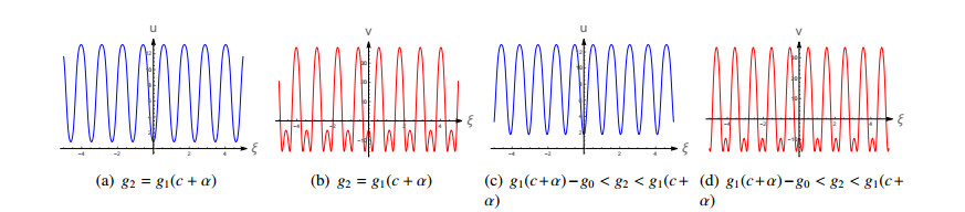
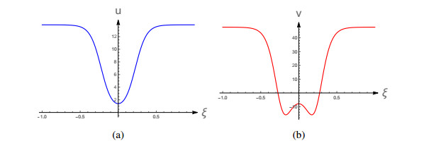
1. | Zhenshu Wen, Huijun Li, Yanggeng Fu, Abundant explicit periodic wave solutions and their limit forms to space‐time fractional Drinfel'd–Sokolov–Wilson equation, 2021, 0170-4214, 10.1002/mma.7192 | |
2. | Mei Xu, Bo Du, New approaches for periodic wave solutions of a non-Newtonian filtration equation with variable delay, 2021, 2021, 1687-2770, 10.1186/s13661-021-01492-y | |
3. | Lin Lu, Xiaokai He, Aiyong Chen, Monotonicity of the period function of periodic standing waves for nearly parallel vortex filaments model, 2025, 1468-9367, 1, 10.1080/14689367.2025.2454447 |