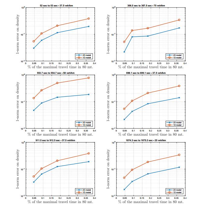
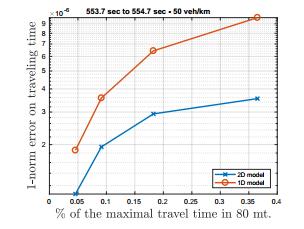
Based on experimental traffic data obtained from German and US highways, we propose a novel two-dimensional first-order macroscopic traffic flow model. The goal is to reproduce a detailed description of traffic dynamics for the real road geometry. In our approach both the dynamics along the road and across the lanes is continuous. The closure relations, being necessary to complete the hydrodynamics equation, are obtained by regression on fundamental diagram data. Comparison with prediction of one-dimensional models shows the improvement in performance of the novel model.
Citation: Michael Herty, Adrian Fazekas, Giuseppe Visconti. A two-dimensional data-driven model for traffic flow on highways[J]. Networks and Heterogeneous Media, 2018, 13(2): 217-240. doi: 10.3934/nhm.2018010
Based on experimental traffic data obtained from German and US highways, we propose a novel two-dimensional first-order macroscopic traffic flow model. The goal is to reproduce a detailed description of traffic dynamics for the real road geometry. In our approach both the dynamics along the road and across the lanes is continuous. The closure relations, being necessary to complete the hydrodynamics equation, are obtained by regression on fundamental diagram data. Comparison with prediction of one-dimensional models shows the improvement in performance of the novel model.

| [1] | Federal Highway Administration US Department of Transportation. Next Generation Simulation (NGSIM), Available from: http://ops.fhwa.dot.gov/trafficanalysistools/ngsim.htm. |
| [2] | Minnesota Department of Transportation. Mn/DOT Traffic Data, Available from: http://data.dot.state.mn.us/datatools. |
| [3] | Mobile Millennium Project, Available from: http://traffic.berkeley.edu. |
| [4] | 75 Years of the Fundamental Diagram for Traffic Flow Theory: Greenshields Symposium, Transportation Research Board, Circular E-C149. 2011. |
| [5] | S. Amin et al., Mobile century – Using GPS mobile phones as traffic sensors: A field experiment. 15th World Congress on Intelligent Transportation Systems, New York. Nov. 2008. |
| [6] |
Discrete Kinetic Schemes for Multidimensional Conservation Laws. SIAM J. Numer. Anal. (2000) 37: 1973-2004. 
|
| [7] |
Resurrection of "second order" models of traffic flow. SIAM J. Appl. Math. (2000) 60: 916-938 (electronic).
|
| [8] |
Lax-Hopf based incorporation of internal boundary conditions into Hamilton-Jacobi equation. Part Ⅰ: Theory. IEEE Trans. Automat. Contr. (2010) 55: 1142-1157.
|
| [9] |
Convex formulations of data assimilation problems for a class of hamilton-jacobi equations. SIAM J. Control Optim. (2011) 49: 383-402.
|
| [10] |
On the modeling of traffic and crowds: A survey of models, speculations, and perspectives. SIAM Rev. (2011) 53: 409-463.
|
| [11] |
An
|
| [12] |
A model for the formation and evolution of traffic jams. Arch. Ration. Mech. Anal. (2008) 187: 185-220.
|
| [13] |
Numerical simulations of traffic data via fluid dynamic approach. Appl. Math. Comput. (2009) 210: 441-454.
|
| [14] |
A comparative study of several smoothing methods in density estimation. Comput. Stat. Data. An. (1994) 17: 153-176.
|
| [15] | B. N. Chetverushkin, N. G. Churbanova, I. R. Furmanov and M. A. Trapeznikova, 2D Micro-and Macroscopic Models for Simulation of Heterogeneous Traffic Flows, Proceedings of the ECCOMAS CFD 2010, V European Conference on Computational Fluid Dynamics, 2010. |
| [16] | B. N. Chetverushkin, N. G. Churbanova, A. B. Sukhinova and M. A. Trapeznikova, Congested Traffic Simulation Based on a 2D Hydrodynamical Model, Proceedings of 8th World Congress on Computational Mechanics and 5th European Congress on Computational Methods in Applied Science and Engineering, WCCM8 & ECCOMAS, 2008. |
| [17] |
Über die partiellen Differenzengleichungen der mathematischen Physik. Mathematische Annalen (1928) 100: 32-74.
|
| [18] |
CWENO: Uniformly accurate reconstructions for balance laws. Math. Comp. (2018) 87: 1689-1719.
|
| [19] |
The cell transmission model: A dynamic representation of highway traffic consistent with the hydrodynamic theory. Transport. Res. B-Meth. (1994) 28: 269-287.
|
| [20] |
Requiem for second order fluid approximations of traffic flow. Transport. Res. B-Meth. (1995) 29: 277-286.
|
| [21] |
In traffic flow, cellular automata = kinematic waves. Transport. Res. B-Meth. (2006) 40: 396-403.
|
| [22] |
Comparative model accuracy of a data-fitted generalized Aw-Rascle-Zhang model. Netw. Heterog. Media (2014) 9: 239-268.
|
| [23] | S. Fan and B. Seibold, A comparison of data-fitted first order traffic models and their second order generalizations via trajectory and sensor data, arXiv: 1208.0382, (2012). |
| [24] | M. Garavello and B. Piccoli, Traffic Flow on Networks, AIMS Series on Applied Mathematics, American Institute of Mathematical Sciences (AIMS), Springfield, MO, 2006. |
| [25] |
The Aw-Rascle vehicular traffic flow model with phase transitions. Math. Comput. Modeling (2006) 44: 287-303.
|
| [26] | Finite difference methods for numerical computation of discontinuous solutions of the equations of fluid dynamics. Mat. Sbornik (1959) 47: 271-306. |
| [27] | A study of traffic capacity. Proc. Highway Res. (1935) 14: 448-477. |
| [28] |
High resolution schemes for hyperbolic conservation laws. J. Comp. Phys. (1983) 49: 357-393.
|
| [29] |
Traffic and related self-driven many-particle systems. Reviews of Modern Physics (2001) 73: 1067-1141.
|
| [30] |
Analytical and numerical investigations of refined macroscopic traffic flow models. Kinet. Relat. Models (2010) 3: 311-333.
|
| [31] |
Fokker-Planck asymptotics for traffic flow models. Kinet. Relat. Models (2010) 3: 165-179.
|
| [32] | M. Herty, S. Moutari and G. Visconti, Macroscopic modeling of multi-lane motorways using a two-dimensional second-order model of traffic flow, Submitted, arXiv: 1710.07209, (2017). |
| [33] | M. Herty, A. Tosin, G. Visconti and M. Zanella, Hybrid stochastic kinetic description of two-dimensional traffic dynamics, Submitted, arXiv: 1711.02424, (2017). |
| [34] | M. Herty and G. Visconti, Analysis of risk levels for traffic on a multi-lane highway, Submitted, arXiv: 1710. 05752, (2017). |
| [35] | Neue Methoden zur approximativen Integration der Differentialgleichungen einer unabhängigen Veränderlichen. Z. Math. Phys (1900) 45: 23-38. |
| [36] | S. P. Hoogendoorn, Traffic Flow Theory and Simulation: CT4821, Delft University of Technology, Faculty of Civil Engineering and Geosciences (TU Delft), 2007. |
| [37] |
R. Illner, A. Klar and T. Materne, Vlasov-Fokker-Planck models for multilane traffic
flow, Commun. Math. Sci., 1 (2003), 1–12, URL http://projecteuclid.org/euclid.cms/1118150395. doi: 10.4310/CMS.2003.v1.n1.a1
|
| [38] |
A brief survey of bandwidth selection for density estimation. J. Am. Statist. Assoc. (1996) 91: 401-407.
|
| [39] |
B. S. Kerner,
The Physics of Traffic, Understanding Complex Systems. Springer, Berlin, 2004. doi: 10.1007/978-3-540-40986-1
|
| [40] |
Cluster effect in initially homogeneous traffic flow. Phys. Rev. E (1993) 48: R2335-R2338.
|
| [41] |
Structure and parameters of clusters in traffic flow. Phys. Rev. E (1994) 50: 54-83.
|
| [42] |
A hierarchy of models for multilane vehicular traffic. Ⅰ. Modeling. SIAM J. Appl. Math. (1999) 59: 983-1001 (electronic).
|
| [43] |
A hierarchy of models for multilane vehicular traffic. Ⅱ. Numerical investigations. SIAM J. Appl. Math. (1999) 59: 1002-1011 (electronic).
|
| [44] |
Kinetic derivation of macroscopic anticipation models for vehicular traffic. SIAM J. Appl. Math. (2000) 60: 1749-1766 (electronic).
|
| [45] | Les modeles macroscopiques du traffic. Annales des Ponts. (1993) 67: 24-45. |
| [46] |
W. Leutzbach,
Introduction to the Theory of Traffic Flow, Springer, New York, 1988. doi: 10.1007/978-3-642-61353-1
|
| [47] |
R. J. LeVeque,
Finite-Volume Methods for Hyperbolic Problems, Cambridge University Press, Cambridge, 2002. doi: 10.1017/CBO9780511791253
|
| [48] |
On kinematic waves. Ⅱ. A theory of traffic flow on long crowded roads. Proc. Roy. Soc. London. Ser. A. (1955) 229: 317-345.
|
| [49] | S. Maerivoet and B. De Moor, Traffic Flow Theory, Katholieke Universiteit Leuven, 2005. |
| [50] |
A simplified theory of kinematic waves in highway traffic Ⅱ: Queueing at freeway bottlenecks. Transport. Res. B-Meth. (1993) 27: 289-303.
|
| [51] |
On estimation of a probability density function and model. Ann. Math. Statist. (1962) 33: 1065-1076.
|
| [52] | Models of freeway traffic and control. Math. Models Publ. Sys., Simul. Council Proc. (1971) 28: 51-61. |
| [53] | FREFLO: A macroscopic simulation model for freeway traffic. Transportation Research Record (1979) 722: 68-77. |
| [54] |
A kinetic model for traffic flow with continuum implications. Transportation Planning and Technology (1979) 5: 131-138.
|
| [55] |
B. Piccoli and A. Tosin, Vehicular traffic: A review of continuum mathematical models, in
Mathematics of Complexity and Dynamical Systems. Vols. 1–3, Springer, New York, 2012,
1748–1770. doi: 10.1007/978-1-4614-1806-1_112
|
| [56] | I. Prigogine and R. Herman, Kinetic Theory of Vehicular Traffic, American Elsevier Publishing Co., New York, 1971. |
| [57] |
Fundamental diagrams in traffic flow: The case of heterogeneous kinetic models. Commun. Math. Sci. (2016) 14: 643-669.
|
| [58] |
Analysis of a multi-population kinetic model for traffic flow. Commun. Math. Sci. (2017) 15: 379-412.
|
| [59] |
Shock waves on the highway. Operations Res. (1956) 4: 42-51.
|
| [60] |
Remarks on some nonparametric estimates of a density function. Ann. Math. Statist. (1956) 27: 832-837.
|
| [61] |
M. D. Rosini,
Macroscopic Models for Vehicular Flows and Crowd Dynamics: Theory and Applications, Understanding Complex Systems, Springer, Heidelberg, 2013. doi: 10.1007/978-3-319-00155-5
|
| [62] |
High order weighted essentially nonoscillatory schemes for convection dominated problems. SIAM Rev. (2009) 51: 82-126.
|
| [63] |
On the construction and comparison of difference schemes. SIAM J. Numer. Anal. (1968) 5: 506-517.
|
| [64] |
Two-dimensional macroscopic model of traffic flows. Mathematical Models and Computer Simulations (2009) 1: 669-676.
|
| [65] |
E. F. Toro,
Riemann Solvers and Numerical Methods for Fluid Dynamics, Springer, Berlin, 2009. doi: 10.1007/b79761
|
| [66] | R. T. Underwood, Speed, Volume, And Density Relationships: Quality and theory of traffic flow, Yale Bureau of Highway Traffic, (1961), 141–188. |
| [67] | Towards the ultimate conservative difference scheme Ⅲ. Upstream-centered finite-difference schemes for ideal compressible flow. J. Comp. Phys. (1977) 23: 263-275. |
| [68] |
A non-equilibrium traffic model devoid of gas-like behavior. Transport. Res. B-Meth. (2002) 36: 275-290.
|
Figures(12)
Michael Herty, Adrian Fazekas, Giuseppe Visconti. A two-dimensional data-driven model for traffic flow on highways[J]. Networks and Heterogeneous Media, 2018, 13(2): 217-240. doi: 10.3934/nhm.2018010


 DownLoad: