A macroscopic traffic model with phase transitions and local point constraints on the flow

Mohamed Benyahia; Massimiliano D. Rosini; Mohamed Benyahia; Massimiliano D. Rosini

doi:10.3934/nhm.2017013

Networks and Heterogeneous Media

2017, Volume 12, Issue 2: 297-317. doi: 10.3934/nhm.2017013

Previous Article Next Article

A macroscopic traffic model with phase transitions and local point constraints on the flow

Mohamed Benyahia ^{1
,},
Massimiliano D. Rosini ^{2
,
,}

1.
Gran Sasso Science Institute, Viale F. Crispi 7,67100 L'Aquila, Italy
2.
Instytut Matematyki, Uniwersytet Marii Curie-Skłodowskiej, Plac Marii Curie-Skłodowskiej 1, 20-031 Lublin, Poland

Received: 01 November 2016 Revised: 01 January 2017
Primary: 35L65, 90B20; Secondary: 82C26

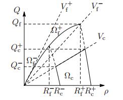
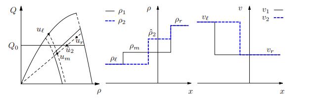
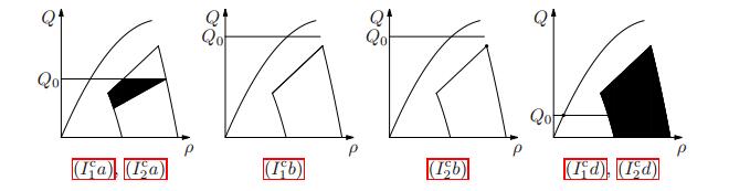
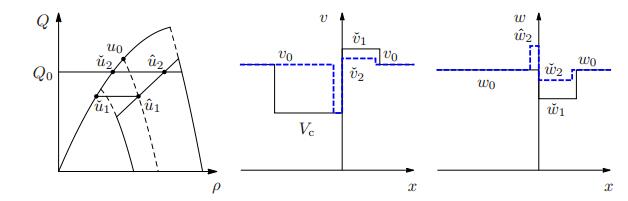
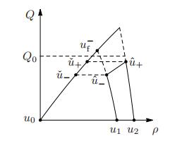
In this paper we present a macroscopic phase transition model with a local point constraint on the flow. Its motivation is, for instance, the modelling of the evolution of vehicular traffic along a road with pointlike inhomogeneities characterized by limited capacity, such as speed bumps, traffic lights, construction sites, toll booths, etc. The model accounts for two different phases, according to whether the traffic is low or heavy. Away from the inhomogeneities of the road the traffic is described by a first order model in the free-flow phase and by a second order model in the congested phase. To model the effects of the inhomogeneities we propose two Riemann solvers satisfying the point constraints on the flow.
- Conservation laws,
- phase transitions,
- Lighthill-Whitham-Richards model,
- Aw-Rascle-Zhang model,
- unilateral constraint,
- Riemann problem
Citation: Mohamed Benyahia, Massimiliano D. Rosini. A macroscopic traffic model with phase transitions and local point constraints on the flow[J]. Networks and Heterogeneous Media, 2017, 12(2): 297-317. doi: 10.3934/nhm.2017013

Related Papers:

Abstract

In this paper we present a macroscopic phase transition model with a local point constraint on the flow. Its motivation is, for instance, the modelling of the evolution of vehicular traffic along a road with pointlike inhomogeneities characterized by limited capacity, such as speed bumps, traffic lights, construction sites, toll booths, etc. The model accounts for two different phases, according to whether the traffic is low or heavy. Away from the inhomogeneities of the road the traffic is described by a first order model in the free-flow phase and by a second order model in the congested phase. To model the effects of the inhomogeneities we propose two Riemann solvers satisfying the point constraints on the flow.

References

[1]	Riemann problems with non-local point constraints and capacity drop. Math. Biosci. Eng. (2015) 12: 259-278.
[2]	Qualitative behaviour and numerical approximation of solutions to conservation laws with non-local point constraints on the flux and modeling of crowd dynamics at the bottlenecks. ESAIM: M2AN (2016) 50: 1269-1287.
[3]	Crowd dynamics and conservation laws with nonlocal constraints and capacity drop. Math. Models Methods Appl. Sci. (2014) 24: 2685-2722.
[4]	A second-order model for vehicular traffics with local point constraints on the flow. Math. Models Methods Appl. Sci. (2016) 26: 751-802.
[5]	Finite volume schemes for locally constrained conservation laws. Numer. Math. (2010) 115: 609-645, With supplementary material available online.
[6]	Solutions of the Aw-Rascle-Zhang system with point constraints. Netw. Heterog. Media (2016) 11: 29-47.
[7]	A. Aw and M. Rascle, Resurrection of "second order" models of traffic flow, SIAM J. Appl. Math., 60 (2000), 916–938 (electronic). doi: 10.1137/S0036139997332099
[8]	On the modeling of traffic and crowds: A survey of models, speculations, and perspectives. SIAM Rev. (2011) 53: 409-463.
[9]	Entropy solutions for a traffic model with phase transitions. Nonlinear Anal. (2016) 141: 167-190.
[10]	A general phase transition model for vehicular traffic. SIAM J. Appl. Math. (2011) 71: 107-127.
[11]	A. Bressan, Hyperbolic Systems of Conservation Laws, vol. 20 of Oxford Lecture Series in Mathematics and its Applications, Oxford University Press, Oxford, 2000, The one-dimensional Cauchy problem.
[12]	Error estimate for Godunov approximation of locally constrained conservation laws. SIAM J. Numer. Anal. (2012) 50: 3036-3060.
[13]	C. Chalons and P. Goatin, Computing phase transitions arising in traffic flow modeling, in Hyperbolic Problems: Theory, Numerics, Applications, Springer, Berlin, 2008,559–566. doi: 10.1007/978-3-540-75712-2_54
[14]	Godunov scheme and sampling technique for computing phase transitions in traffic flow modeling. Interfaces Free Bound. (2008) 10: 197-221.
[15]	General constrained conservation laws. Application to pedestrian flow modeling. Netw. Heterog. Media (2013) 8: 433-463.
[16]	Phase transition model for traffic at a junction. J. Math. Sci. (N. Y.) (2014) 196: 30-36.
[17]	R. M. Colombo, Hyperbolic phase transitions in traffic flow, SIAM J. Appl. Math., 63 (2002), 708–721 (electronic). doi: 10.1137/S0036139901393184
[18]	R. M. Colombo, Phase transitions in hyperbolic conservation laws, in Progress in Analysis, Vol. I, II (Berlin, 2001), World Sci. Publ., River Edge, NJ, 2003,1279–1287.
[19]	A well posed conservation law with a variable unilateral constraint. J. Differential Equations (2007) 234: 654-675.
[20]	Road networks with phase transitions. J. Hyperbolic Differ. Equ. (2010) 7: 85-106.
[21]	Global well posedness of traffic flow models with phase transitions. Nonlinear Anal. (2007) 66: 2413-2426.
[22]	On the modelling and management of traffic. ESAIM Math. Model. Numer. Anal. (2011) 45: 853-872.
[23]	A 2-phase traffic model based on a speed bound. SIAM J. Appl. Math. (2010) 70: 2652-2666.
[24]	E. Dal Santo, M. D. Rosini, N. Dymski and M. Benyahia, General phase transition models for vehicular traffic with point constraints on the flow, arXiv preprint, arXiv: 1608.04932.
[25]	The Aw-Rascle traffic model with locally constrained flow. J. Math. Anal. Appl. (2011) 378: 634-648.
[26]	M. Garavello and S. Villa, The Cauchy problem for the Aw-Rascle-Zhang traffic model with locally constrained flow, 2016, URL https://www.math.ntnu.no/conservation/2016/007.pdf.
[27]	M. Garavello, K. Han and B. Piccoli, Models for Vehicular Traffic on Networks, vol. 9 of AIMS Series on Applied Mathematics, American Institute of Mathematical Sciences (AIMS), Springfield, MO, 2016, Conservation laws models.
[28]	Traffic flow on a road network using the Aw-Rascle model. Comm. Partial Differential Equations (2006) 31: 243-275.
[29]	M. Garavello and B. Piccoli, Traffic Flow on Networks, vol. 1 of AIMS Series on Applied Mathematics, American Institute of Mathematical Sciences (AIMS), Springfield, MO, 2006, Conservation laws models.
[30]	Coupling of Lighthill-Whitham-Richards and phase transition models. J. Hyperbolic Differ. Equ. (2013) 10: 577-636.
[31]	Coupling of microscopic and phase transition models at boundary. Netw. Heterog. Media (2013) 8: 649-661.
[32]	The Aw-Rascle vehicular traffic flow model with phase transitions. Math. Comput. Modelling (2006) 44: 287-303.
[33]	Traffic flow models with phase transitions on road networks. Netw. Heterog. Media (2009) 4: 287-301.
[34]	H. Holden and N. H. Risebro, Front Tracking for Hyperbolic Conservation Laws, vol. 152 of Applied Mathematical Sciences, 2nd edition, Springer, Heidelberg, 2015. doi: 10.1007/978-3-662-47507-2
[35]	M. J. Lighthill and G. B. Whitham, On kinematic waves. Ⅱ. A theory of traffic flow on long crowded roads, in Proceedings of the Royal Society. London. Series A. Mathematical, Physical and Engineering Sciences, 229 (1955), 317–345. doi: 10.1098/rspa.1955.0089
[36]	State-of-the art of macroscopic traffic flow modelling. Int. J. Adv. Eng. Sci. Appl. Math. (2013) 5: 158-176.
[37]	The generalized Riemann problem for the Aw-Rascle model with phase transitions. J. Math. Anal. Appl. (2012) 389: 685-693.
[38]	The global solution of the interaction problem for the Aw-Rascle model with phase transitions. Math. Methods Appl. Sci. (2012) 35: 1700-1711.
[39]	B. Piccoli and A. Tosin, Vehicular traffic: A review of continuum mathematical models, in Mathematics of complexity and dynamical systems. Vols. 1–3, Springer, New York, 2012, 1748–1770. doi: 10.1007/978-1-4614-1806-1_112
[40]	Shock waves on the highway. Operations Res. (1956) 4: 42-51.
[41]	The initial-boundary value problem and the constraint. Macroscopic Models for Vehicular Flows and Crowd Dynamics: Theory and Applications (2013) 63-91.
[42]	M. D. Rosini, Macroscopic Models for Vehicular Flows and Crowd Dynamics: Theory and Applications, Understanding Complex Systems, Springer, Heidelberg, 2013. doi: 10.1007/978-3-319-00155-5
[43]	A non-equilibrium traffic model devoid of gas-like behavior. Transportation Research Part B: Methodological (2002) 36: 275-290.

Reader Comments

Your name:*

Email:*
© 2017 the Author(s), licensee AIMS Press. This is an open access article distributed under the terms of the Creative Commons Attribution License (http://creativecommons.org/licenses/by/4.0)