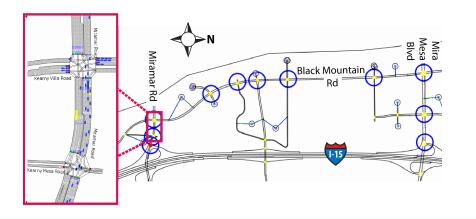
Intelligent use of network capacity via responsive signal control will become increasingly essential as congestion increases on urban roadways. Existing adaptive control systems require lengthy location-specific tuning procedures or expensive central communications infrastructure. Previous theoretical work proposed the application of a max pressure controller to maximize network throughput in a distributed manner with minimal calibration. Yet this algorithm as originally formulated has unpractical hardware and safety constraints. We fundamentally alter the formulation of the max pressure controller to a setting where the actuation can only update once per multiple time steps of the modeled dynamics. This is motivated by the case of a traffic signal that can only update green splits based on observed link-counts once per "cycle time" of 60-120 seconds. Furthermore, we extend the domain of allowable actuations from a single signal phase to any convex combination of available signal phases to model intra-cycle signal changes dictated by pre-selected cycle green splits. We show that this extended max pressure controller will stabilize a vertical queueing network given restrictions on admissible demand flows that are slightly stronger than those suggested in the original formulation of max pressure. We ultimately apply our cycle-based extension of max pressure to a simulation of an existing arterial network and provide comparison to the control policy that is currently deployed at the modeled location.
Citation: Leah Anderson, Thomas Pumir, Dimitrios Triantafyllos, Alexandre M. Bayen. Stability and implementation of a cycle-based max pressure controller for signalized traffic networks[J]. Networks and Heterogeneous Media, 2018, 13(2): 241-260. doi: 10.3934/nhm.2018011
Intelligent use of network capacity via responsive signal control will become increasingly essential as congestion increases on urban roadways. Existing adaptive control systems require lengthy location-specific tuning procedures or expensive central communications infrastructure. Previous theoretical work proposed the application of a max pressure controller to maximize network throughput in a distributed manner with minimal calibration. Yet this algorithm as originally formulated has unpractical hardware and safety constraints. We fundamentally alter the formulation of the max pressure controller to a setting where the actuation can only update once per multiple time steps of the modeled dynamics. This is motivated by the case of a traffic signal that can only update green splits based on observed link-counts once per "cycle time" of 60-120 seconds. Furthermore, we extend the domain of allowable actuations from a single signal phase to any convex combination of available signal phases to model intra-cycle signal changes dictated by pre-selected cycle green splits. We show that this extended max pressure controller will stabilize a vertical queueing network given restrictions on admissible demand flows that are slightly stronger than those suggested in the original formulation of max pressure. We ultimately apply our cycle-based extension of max pressure to a simulation of an existing arterial network and provide comparison to the control policy that is currently deployed at the modeled location.

| [1] |
Store-and-forward based methods for the signal control problem in large-scale congested urban networks. Transportation Research Part C: Emerging Technologies (2009) 17: 163-174. 
|
| [2] |
Estimating the traffic capacity of a signalized road junction. Transportation Research (1972) 6: 245-255.
|
| [3] |
Scheduling in a queuing system with asynchronously varying service rates. Probability in the Engineering and Informational Sciences (2004) 18: 191-217.
|
| [4] |
R. Brockett, Stabilization of motor networks, in Proceedings of the 34th IEEE Conference on
Decision and Control, 1995, 1484–1488. doi: 10.1109/CDC.1995.480312
|
| [5] |
Maximum pressure policies in stochastic processing networks. Operations Research (2005) 53: 197-218.
|
| [6] |
Decentralized control of traffic networks. IEEE Transactions on Systems, Man, and Cybernetics (1983) 13: 476-487.
|
| [7] |
M. Egerstedt and Y. Wardi, Multi-process control using queuing theory, in Proceedings of the
41st IEEE Conference on Decision and Control, 2002, 1991–1996. doi: 10.1109/CDC.2002.1184820
|
| [8] |
P. Giaccone, E. Leonardi and D. Shah, On the maximal throughput of networks with finite
buffers and its application to buffered crossbars, in Proceedings of the 24th Annual Joint
Conference of the IEEE Computer and Communications Societies, 2005,971–980. doi: 10.1109/INFCOM.2005.1498326
|
| [9] | P. B. Hunt, D. I. Robertson, R. D. Bretherton and R. I. Winton, SCOOT - a Traffic Responsive Method of Coordinating Signals, Transport and Road Research Laboratory, UK, 1981. |
| [10] |
Stabilizing a linear system by switching control with dwell time. IEEE Trans. Automat. Control (2002) 47: 1962-1973.
|
| [11] | Dynamic power allocation and routing for time-varying wireless networks. IEEE Journal on Selected Areas in Communications (2005) 23: 89-103. |
| [12] |
M. Pajic, S. Sundaram and G. J. Pappas,
Stabilizability over Deterministic Relay Networks, in Proceedings of the 52nd IEEE Conference on Decision and Control, 2013. doi: 10.1109/CDC.2013.6760504
|
| [13] |
The Sydney coordinated adaptive traffic (SCAT) system philosophy and benefits. IEEE Transactions on Vehicular Technology (1980) 29: 130-137.
|
| [14] |
MaxWeight scheduling in a generalized switch: State space collapse and workload minimization in heavy traffic. Annals of Applied Probability (2004) 14: 1-53.
|
| [15] |
Adaptive back-pressure congestion control-based on local information. IEEE Transactions on Automatic Control (1995) 40: 236-250.
|
| [16] |
Stability properties of constrained queueing systems and scheduling policies for maximum throughput in multihop radio networks. IEEE Transactions on Automatic Control (1992) 37: 1936-1948.
|
| [17] | M. van den Berg, A. Hegyi, B. De Schutter and H. Hellendoorn, A macroscopic traffic flow model for integrated control of freeway and urban traffic networks, in Proceedings of the 42nd IEEE Conference on Decision and Control, 2003, 2774–2779. |
| [18] |
Max pressure control of a network of signalized intersections. Transportation Research Part C: Emerging Technologies (2013) 36: 177-195.
|
| [19] |
T. Wongpiromsarn, T. Uthaicharoenpong, Y. Wang, E. Frazzoli and D. Wang, Distributed
traffic signal control for maximum network throughput, in Proceedings of the 15th International IEEE Conference on Intelligent Transportation Systems, 2012,588–595. doi: 10.1109/ITSC.2012.6338817
|
| [20] | Modelling network flow with and without link interactions: The cases of point queue, spatial queue and cell transmission model. Transportmetrica B: Transport Dynamics (2013) 1: 33-51. |
Figures(5)
Leah Anderson, Thomas Pumir, Dimitrios Triantafyllos, Alexandre M. Bayen. Stability and implementation of a cycle-based max pressure controller for signalized traffic networks[J]. Networks and Heterogeneous Media, 2018, 13(2): 241-260. doi: 10.3934/nhm.2018011


 DownLoad: