An improved pix2pix model based on Gabor filter for robust color image rendering

Hong-an Li; Min Zhang; Zhenhua Yu; Zhanli Li; Na Li; Hong-an Li; Min Zhang; Zhenhua Yu; Zhanli Li; Na Li

doi:10.3934/mbe.2022004

Mathematical Biosciences and Engineering

2022, Volume 19, Issue 1: 86-101. doi: 10.3934/mbe.2022004

Previous Article Next Article

Research article Special Issues

An improved pix2pix model based on Gabor filter for robust color image rendering

College of Computer Science and Technology, Xi'an University of Science and Technology, Xi'an 710054, China

Academic Editor:Tsang-Chuan Chang

Received: 02 September 2021 Accepted: 27 October 2021 Published: 08 November 2021

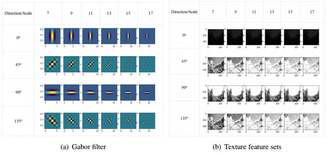
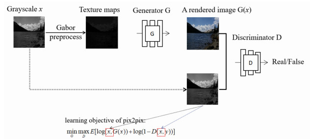
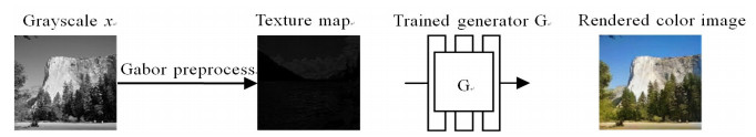
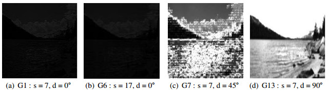
In recent years, with the development of deep learning, image color rendering method has become a research hotspot once again. To overcome the detail problems of color overstepping and boundary blurring in the robust image color rendering method, as well as the problems of unstable training based on generative adversarial networks, we propose an color rendering method using Gabor filter based improved pix2pix for robust image. Firstly, the multi-direction/multi-scale selection characteristic of Gabor filter is used to preprocess the image to be rendered, which can retain the detailed features of the image while preprocessing to avoid the loss of features. Moreover, among the Gabor texture feature maps with 6 scales and 4 directions, the texture map with the scale of 7 and the direction of 0° has the comparable rendering performance. Finally, by improving the loss function of pix2pix model and adding the penalty term, not only the training can be stabilized, but also the ideal color image can be obtained. To reflect image color rendering quality of different models more objectively, PSNR and SSIM indexes are adopted to evaluate the rendered images. The experimental results of the proposed method show that the robust image rendered by this method has better visual performance and reduces the influence of light and noise on the image to a certain extent.

Keywords:

Citation: Hong-an Li, Min Zhang, Zhenhua Yu, Zhanli Li, Na Li. An improved pix2pix model based on Gabor filter for robust color image rendering[J]. Mathematical Biosciences and Engineering, 2022, 19(1): 86-101. doi: 10.3934/mbe.2022004

Related Papers:

[1]	Xiaoxue Zhao, Zhuchun Li . Synchronization of a Kuramoto-like model for power grids with frustration. Networks and Heterogeneous Media, 2020, 15(3): 543-553. doi: 10.3934/nhm.2020030
[2]	Tingting Zhu . Synchronization of the generalized Kuramoto model with time delay and frustration. Networks and Heterogeneous Media, 2023, 18(4): 1772-1798. doi: 10.3934/nhm.2023077
[3]	Seung-Yeal Ha, Yongduck Kim, Zhuchun Li . Asymptotic synchronous behavior of Kuramoto type models with frustrations. Networks and Heterogeneous Media, 2014, 9(1): 33-64. doi: 10.3934/nhm.2014.9.33
[4]	Tingting Zhu . Emergence of synchronization in Kuramoto model with frustration under general network topology. Networks and Heterogeneous Media, 2022, 17(2): 255-291. doi: 10.3934/nhm.2022005
[5]	Seung-Yeal Ha, Jaeseung Lee, Zhuchun Li . Emergence of local synchronization in an ensemble of heterogeneous Kuramoto oscillators. Networks and Heterogeneous Media, 2017, 12(1): 1-24. doi: 10.3934/nhm.2017001
[6]	Seung-Yeal Ha, Jeongho Kim, Jinyeong Park, Xiongtao Zhang . Uniform stability and mean-field limit for the augmented Kuramoto model. Networks and Heterogeneous Media, 2018, 13(2): 297-322. doi: 10.3934/nhm.2018013
[7]	Seung-Yeal Ha, Hansol Park, Yinglong Zhang . Nonlinear stability of stationary solutions to the Kuramoto-Sakaguchi equation with frustration. Networks and Heterogeneous Media, 2020, 15(3): 427-461. doi: 10.3934/nhm.2020026
[8]	Seung-Yeal Ha, Se Eun Noh, Jinyeong Park . Practical synchronization of generalized Kuramoto systems with an intrinsic dynamics. Networks and Heterogeneous Media, 2015, 10(4): 787-807. doi: 10.3934/nhm.2015.10.787
[9]	Vladimir Jaćimović, Aladin Crnkić . The General Non-Abelian Kuramoto Model on the 3-sphere. Networks and Heterogeneous Media, 2020, 15(1): 111-124. doi: 10.3934/nhm.2020005
[10]	Young-Pil Choi, Seung-Yeal Ha, Seok-Bae Yun . Global existence and asymptotic behavior of measure valued solutions to the kinetic Kuramoto--Daido model with inertia. Networks and Heterogeneous Media, 2013, 8(4): 943-968. doi: 10.3934/nhm.2013.8.943

Abstract

1. Introduction

Synchronization in complex networks has been a focus of interest for researchers from different disciplines[1,2,4,8,15]. In this paper, we investigate synchronous phenomena in an ensemble of Kuramoto-like oscillators which is regarded as a model for power grid. In [9], a mathematical model for power grid is given by

$\begin{equation} P_{source}^{i} = I\ddot{\theta}_{i}\dot{\theta}_{i}+K_{D}(\dot{\theta}_{i})^2-\sum\limits_{l = 1}^{N}a_{il}\sin(\theta_{l}-\theta_{i}),\quad i = 1,2,\dots,N, \end{equation}$

(1)

where $P_{source}^{i}>0$ is power source (the energy feeding rate) of the $i$ th node, $I\ge 0$ is the moment of inertia, $K_{D}>0$ is the ratio between the dissipated energy by the turbine and the square of the angular velocity, and $a_{il}>0$ is the maximum transmitted power between the $i$ th and $l$ th nodes. The phase angle $\theta_{i}$ of $i$ th node is given by $\theta_i(t) = \Omega t+\tilde\theta_i(t)$ with a standard frequency $\Omega$ (50 or 60 Hz) and small deviations $\tilde\theta_i(t)$ . Power plants in a big connected network should be synchronized to the same frequency. If loads are too strong and unevenly distributed or if some major fault or a lightening occurs, an oscillator (power plant) may lose synchronization. In that situation the synchronization landscape may change drastically and a blackout may occur. The transient stability of power grids can be regarded as a synchronization problem for nonstationary generator rotor angles aiming to restore synchronism subject to local excitations. Therefore, the region of attraction of synchronized states is a central problem for the transient stability.

By denoting $\omega_{i} = \frac{P_{source}^{i}}{K_{D}}$ and assuming $\frac{a_{il}}{K_{D}} = \frac{K}{N} \,(\forall i,l\in\{1,2,\dots,N\})$ and $I = 0$ in (1), Choi et. al derived a Kuramoto-like model for the power grid as follows [5]:

$\begin{equation} (\dot{\theta}_{i})^2 = \omega_{i}+\frac{K}{N}\sum\limits_{l = 1}^{N}\sin(\theta_{l}-\theta_{i}),\quad \dot{\theta}_{i} > 0,\quad i = 1,2,\dots,N. \end{equation}$

(2)

Here, the setting $\dot{\theta}_{i}>0$ was made in accordance to the observation in system (1) that the grid is operating at a frequency close to the standard frequency with small deviations. In order to ensure that the right-hand side of (2) is positive, it is reasonable to assume that $\omega_{i}>K,\; i = 1,2,\dots,N$ . This model can be used to understand the emergence of synchronization in networks of oscillators. As far as the authors know, there are few analytical results. In [5], the authors considered this model with identical natural frequencies and prove that complete phase synchronization occurs if the initial phases are distributed inside an arc with geodesic length less than $\pi/2$ .

If $(\dot{\theta}_{i})^2$ in (2) is replaced by $\dot{\theta}_{i}$ , the model is the famous Kuramoto model [13]; for its synchronization analysis we refer to [3,6,10], etc. Sakaguchi and Kuramoto [16] proposed a variant of the Kuramoto model to describe richer dynamical phenomena by introducing a phase shift (frustration) in the coupling function, i.e., by replacing $\sin(\theta_{l}-\theta_{i})$ with $\sin(\theta_{l}-\theta_{i}+\alpha)$ . They inferred the need of $\alpha$ from the empirical fact that a pair of oscillators coupled strongly begin to oscillate with a common frequency deviating from the simple average of their natural frequencies. Some physicists also realized via many experiments that the emergence of the phase shift term requires larger coupling strength $K$ and longer relaxation time to exhibit mutual synchronization compared to the zero phase shift case. This is why we call the phase shift a frustration. The effect of frustration has been intensively studied, for example, [11,12,14]. In power grid model using Kuramoto oscillators, people use the phase shift to depict the energy loss due to the transfer conductance [7]. In this paper, we will incorporate the phase shift term in (2) and study the Kuramoto-like model with frustration $\alpha\in(-\frac{\pi}{4},\frac{\pi}{4})$ :

$\begin{equation} (\dot{\theta}_{i})^2 = \omega_{i}+\frac{K}{N}\sum\limits_{l = 1}^{N}\sin(\theta_{l}-\theta_{i}+\alpha),\quad \dot{\theta}_{i} > 0,\quad i = 1,2,\dots,N. \end{equation}$

(3)

We will find a trapping region such that any nonstationary state located in this region will evolve to a synchronous state.

The contributions of this paper are twofold: First, for identical oscillators without frustration, we show that the initial phase configurations located in the half circle will converge to complete phase and frequency synchronization. This extends the analytical results in [5] in which the initial phase configuration for synchronization needs to be confined in a quarter of circle. Second, we consider the nonidentical oscillators with frustration and present a framework leading to the boundness of the phase diameter and complete frequency synchronization. To the best of our knowledge, this is the first result for the synchronization of (3) with nonidentical oscillators and frustration.

The rest of this paper is organized as follows. In Section 2, we recall the definitions for synchronization and summarize our main results. In Section 3, we give synchronization analysis and prove the main results. Finally, Section 4 is devoted to a concluding summary.

Notations. We use the following simplified notations throughout this paper:

$\begin{align*} &\nu_{i}: = \dot{\theta}_{i},\; i = 1,2,\dots,N,\;{\omega: = (\omega_{1},\omega_{2},\dots,\omega_{N})},\\ &\bar{\omega}: = \max\limits_{1\le i\le N}\omega_{i}, \; \underline{\omega}: = \min\limits_{1\le i\le N}\omega_{i}, \; { D(\omega): = \bar{\omega}-\underline{\omega}},\\ & \theta_{M}: = \max\limits_{1\le i\le N}\theta_{i},\; \theta_{m}: = \min\limits_{1\le i\le N}\theta_{i},\; D(\theta): = \theta_{M}-\theta_{m},\\ & \nu_{M}: = \max\limits_{1\le i\le N}\nu_{i},\; \nu_{m}: = \min\limits_{1\le i\le N}\nu_{i},\; D(\nu): = \nu_{M}-\nu_{m},\\ & {\theta_{M}^\nu\in\{\theta_{j}| \nu_{j} = \nu_{M}\},\; \theta_{m}^\nu\in\{\theta_{j}| \nu_{j} = \nu_{m}\}}. \end{align*}$

2. Preliminaries

In this paper, we consider the system

$\begin{align} \begin{aligned} (\dot{\theta}_{i})^2& = \omega_{i}+\frac{K}{N}\sum\limits_{l = 1}^{N}\sin(\theta_{l}-\theta_{i}+\alpha),\quad \dot{\theta}_{i} > 0,\quad \alpha\in(-\frac{\pi}{4},\frac{\pi}{4}),\\ \theta_i(0)& = \theta_i^0,\quad \quad i = 1,2,\dots,N. \end{aligned} \end{align}$

(4)

Next we introduce the concepts of complete synchronization and conclude this introductory section with the main result of this paper.

Definition 2.1. Let $\theta: = (\theta_{1},\theta_{2},\dots,\theta_{N})$ be a dynamical solution to the system (4). We say

1. it exhibits asymptotically complete phase synchronization if

$\begin{equation*} \lim\limits_{t\to \infty}(\theta_{i}(t)-\theta_{j}(t)) = 0, \; \forall i\ne j. \end{equation*}$

2. it exhibits asymptotically complete frequency synchronization if

$\begin{equation*} \lim\limits_{t\to \infty}({\dot \theta}_{i}(t)-{\dot \theta}_{j}(t)) = 0, \; \forall i\ne j. \end{equation*}$

For identical oscillators without frustration, we have the following result.

Theorem 2.2. Let $\theta: = (\theta_{1},\theta_{2},\dots,\theta_{N})$ be a solution to the coupled system (4) with $\alpha = 0,\omega_{i} = \omega_0,i = 1,2,\dots,N$ and $\omega_0>K$ . If the initial configuration

$\begin{equation*} \theta^0\in \mathcal{A}: = \{\theta\in[0,2\pi)^N:\; D(\theta) < \pi\}, \end{equation*}$

then there exits $\lambda_1,\lambda_2>0$ and $t_{0}>0$ such that

$\begin{equation} D(\theta(t))\le D(\theta^0)e^{-\lambda_1 t},\;\,\,\,t\ge 0. \end{equation}$

(5)

and

$\begin{equation} D(\nu(t))\le D(\nu(t_{0}))e^{-\lambda_2(t-t_{0})},\;\,\,\,t\ge t_{0}. \end{equation}$

(6)

Next we introduce the main result for nonidentical oscillators with frustration. For $\bar{\omega}< \frac{1}{2\sin^2|\alpha|}$ , we set

$K_{c}: = \frac{D({\omega})\sqrt{2\bar{\omega}}}{1-\sqrt{2\bar{\omega}}\sin|\alpha|} > 0.$

For suitable parameters, we denote by $D_{1}^{\infty}$ and $D_{*}^{\infty}$ the two angles as follows:

$\begin{align*} &\sin D_{1}^{\infty} = \sin D_{*}^{\infty}: = \frac{\sqrt{\bar{\omega}+K}(D({\omega})+K\sin|\alpha|)}{K\sqrt{\underline{\omega}-K}},\quad 0 < D_{1}^{\infty} < \frac{\pi}{2} < D_{*}^{\infty} < \pi. \end{align*}$

Theorem 2.3. Let $\theta: = (\theta_{1},\theta_{2},\dots,\theta_{N})$ be a solution to the coupled system (4) with $K>K_{c}$ and $[\underline{\omega},\bar{\omega}]\subset \left[K+1,\frac{1}{2\sin^2|\alpha|}\right)$ . If

$\begin{equation*} \theta^0\in \mathcal{B}: = \{\theta\in[0,2\pi)^N\;|\; D(\theta) < D_{*}^{\infty}-|\alpha|\}, \end{equation*}$

then for any small $\varepsilon>0$ with $D_{1}^{\infty}+\varepsilon<\frac{\pi}{2}$ , there exists $\lambda_{3}>0$ and $T>0$ such that

$\begin{equation} D(\nu(t))\le D(\nu(T))e^{-\lambda_{3}(t-T)},\;t\ge T. \end{equation}$

(7)

Remark 1. If the parametric conditions in Theorem 2.3 are fulfilled, the reference angles $D_{1}^{\infty}$ and $D_{*}^{\infty}$ are well-defined. Indeed, because $K>K_{c}$ and $\bar{\omega}<\frac{1}{2\sin^2 |\alpha|}$ , we have

$\begin{equation*} \frac{D({\omega})\sqrt{2\bar{\omega}}}{1-\sqrt{2\bar{\omega}}\sin |\alpha|} < K,\qquad 1-\sqrt{2\bar{\omega}}\sin |\alpha| > 0. \end{equation*}$

This implies

$\begin{equation*} \frac{\sqrt{2\bar{\omega}}(D({\omega})+K\sin|\alpha|)}{K} < 1. \end{equation*}$

Then, by $\underline{\omega}\ge K+1$ and $K\le \bar{\omega}$ we obtain

$\begin{align*} \sin D_{1}^{\infty} = \sin D_{*}^{\infty}: = \frac{\sqrt{\bar{\omega}+K}(D({\omega})+K\sin|\alpha|)}{K\sqrt{\underline{\omega}-K}}\le \frac{\sqrt{2\bar{\omega}}(D({\omega})+K\sin|\alpha|)}{K} < 1. \end{align*}$

Remark 2. In order to make $1<K+1<\frac{1}{2\sin^2|\alpha|}$ , it is necessary to assume $\alpha\in \left(-\frac{\pi}{4},\frac{\pi}{4}\right)$ . This is the reason for the setting $\alpha\in \left(-\frac{\pi}{4},\frac{\pi}{4}\right)$ .

3. Synchronization analysis

3.1. Synchronization estimates: Identical oscillators without frustration

In this subsection we consider the system (4) with identical natural frequencies and zero frustration:

$\begin{equation} (\dot{\theta}_{i})^2 = \omega_0+\frac{K}{N}\sum\limits_{l = 1}^{N}\sin(\theta_{l}-\theta_{i}),\quad \dot{\theta}_{i} > 0,\quad i = 1,2,\dots,N. \end{equation}$

(8)

To obtain the complete synchronization, we need to derive a trapping region. We start with two elementary estimates for the transient frequencies.

Lemma 3.1. Suppose $\theta: = (\theta_{1},\theta_{2},\dots,\theta_{N})$ be a solution to the coupled system (8), then for any $i,j\in\{1,2,\dots,N\},$ we have

$\begin{equation*} (\dot{\theta}_{i}-\dot{\theta}_{j})(\dot{\theta}_{i}+\dot{\theta}_{j}) = \frac{2K}{N}\sum\limits_{l = 1}^{N}\cos(\theta_{l}-\frac{\theta_{i}+\theta_{j}}{2})\sin\frac{\theta_{j}-\theta_{i}}{2}. \end{equation*}$

Proof. It is immediately obtained by (8).

Lemma 3.2. Suppose $\theta: = (\theta_{1},\theta_{2},\dots,\theta_{N})$ be a solution to the coupled system (8) and $\Omega>K$ , then we have

$\begin{equation*} \dot{\theta}_{i}\le \sqrt{\omega_0+K}. \end{equation*}$

Proof. It follows from (8) and $\dot{\theta}_{i}>0$ that we have

$\begin{equation*} (\dot{\theta}_{i})^2 = \omega_0+\frac{K}{N}\sum\limits_{l = 1}^{N}\sin(\theta_{l}-\theta_{i})\le \omega_0 +K. \end{equation*}$

Next we give an estimate for trapping region and prove Theorem 2.2. For this aim, we will use the time derivative of $D(\theta(t))$ and $D(\nu(t))$ . Note that $D(\theta(t))$ is Lipschitz continuous and differentiable except at times of collision between the extremal phases and their neighboring phases. Therefore, for the collision time $t$ at which $D(\theta(t))$ is not differentiable, we can use the so-called Dini derivative to replace the classic derivative. In this manner, we can proceed the analysis with differential inequality for $D(\theta(t))$ . For $D(\nu(t))$ we can proceed in the similar way. In the following context, we will always use the notation of classic derivative for $D(\theta(t))$ and $D(\nu(t))$ .

Lemma 3.3. Let $\theta: = (\theta_{1},\theta_{2},\dots,\theta_{N})$ be a solution to the coupled system (8) and $\Omega>K$ . If the initial configuration $\theta(0)\in \mathcal{A}$ , then $\theta(t)\in \mathcal{A},\; t\ge 0$ .

Proof. For any $\theta^0\in \mathcal A$ , there exists $D^\infty\in (0,\pi)$ such that $D(\theta^0)<D^{\infty}$ . Let

$\begin{align*} \mathcal T: = \left\{T\in[0,+\infty)\,\Big|\,D(\theta(t)) < D^{\infty}, \,\, \forall \,t\in [0,T) \right\}. \end{align*}$

Since $D(\theta^0)<D^{\infty}$ , and $D(\theta(t))$ is a continuous function of $t$ , there exists $\eta>0$ such that

$\begin{equation*} D(\theta(t)) < D^{\infty},\;t\in[0,\eta). \end{equation*}$

Therefore, the set $\mathcal T$ is not empty. Let $T^*: = \sup \mathcal T.$ We claim that

$\begin{equation} T^* = \infty. \end{equation}$

(9)

Suppose to the contrary that $T^*<\infty$ . Then from the continuity of $D(\theta(t))$ , we have

$\begin{align*} D(\theta(t)) < D^{\infty},\;t\in[0,T^*),\quad D(\theta(T^*)) = D^{\infty}. \end{align*}$

We use Lemma 3.1 and Lemma 3.2 to obtain

$\begin{align*} \frac{1}{2}\frac{d}{dt}&D(\theta(t))^2 = D(\theta(t))\frac{d}{dt}D(\theta(t)) = \left(\theta_{M}-\theta_{m}\right)\left(\dot{\theta}_{M}-\dot{\theta}_{m}\right) \\ & = \left(\theta_{M}-\theta_{m}\right)\frac{1}{\dot{\theta}_{M}+\dot{\theta}_{m}}\frac{2K}{N}\sum\limits_{l = 1}^{N}\cos\left(\theta_{l}-\frac{\theta_{M}+\theta_{m}}{2}\right)\sin\left(\frac{\theta_{m}-\theta_{M}}{2}\right)\\ &\le \left(\theta_{M}-\theta_{m}\right)\frac{1}{\dot{\theta}_{M}+\dot{\theta}_{m}}\frac{2K}{N}\sum\limits_{l = 1}^{N}\cos\frac{D^{\infty}}{2}\sin\left(\frac{\theta_{m}-\theta_{M}}{2}\right)\\ &\le \left(\theta_{M}-\theta_{m}\right)\frac{1}{\sqrt{\omega_0+K}}\frac{K}{N}\sum\limits_{l = 1}^{N} \cos\frac{D^{\infty}}{2}\sin\left(\frac{\theta_{m}-\theta_{M}}{2}\right)\\ & = -\frac{2K\cos\frac{D^{\infty}}{2}}{\sqrt{\omega_0+K}}\frac{D(\theta)}{2}\sin\frac{D(\theta)}{2}\\ &\le -\frac{K\cos\frac{D^{\infty}}{2}}{\pi\sqrt{\omega_0+K}}D(\theta)^2, \; t\in[0,T^*). \end{align*}$

Here we used the relations

$\begin{equation*} -\frac{D^{\infty}}{2} < -\frac{D(\theta)}{2}\le \frac{\theta_{l}-\theta_{M}}{2}\le 0 \le \frac{\theta_{l}-\theta_{m}}{2}\le \frac{D(\theta)}{2} < \frac{D^{\infty}}{2} \end{equation*}$

and

$\begin{equation*} x\sin x\ge \frac{2}{\pi}x^2,\; x\in\left[-\frac{\pi}{2},\frac{\pi}{2}\right]. \end{equation*}$

Therefore, we have

$\begin{equation} \frac{d}{dt}D(\theta)\le -\frac{K\cos\frac{D^{\infty}}{2}}{\pi\sqrt{\omega_0+K}}D(\theta), \; t\in[0,T^*), \end{equation}$

(10)

which implies that

$\begin{align*} D(\theta(T^*))\le D(\theta^0)e^{-\frac{K\cos\frac{D^{\infty}}{2}}{\pi\sqrt{\omega_0+K}}T^*} < D(\theta^0) < D^{\infty}. \end{align*}$

This is contradictory to $D(\theta(T^*)) = D^{\infty}.$ The claim (9) is proved, which yields the desired result.

Now we can give a proof for Theorem 2.2.

Proof of Theorem 2.2.. According to Lemma 3.3, we substitute $T^* = \infty$ into (10), then (5) is proved with $\lambda_1 = \frac{K\cos\frac{D^{\infty}}{2}}{\pi\sqrt{\omega_0+K}}$ .

On the other hand, by (5) there exist $t_{0}$ and $\delta (0<\delta<\frac{\pi}{2})$ such that $D(\theta(t))\le \delta$ for $t\ge t_{0}$ . Now we differentiate (8) to find

$\begin{equation*} \dot{\nu}_{i} = \frac{K}{2N\nu_{i}}\sum\limits_{l = 1}^{N}\cos(\theta_{l}-\theta_{i})(\nu_{l}-\nu_{i}). \end{equation*}$

Using Lemma 3.2, we now consider the temporal evolution of $D(\nu(t))$ :

$\begin{align*} \frac{d}{dt}&D(\nu) = \dot{\nu}_{M}-\dot{\nu}_{m}\\ & = \frac{K}{2N\nu_{M}}\sum\limits_{l = 1}^{N}\cos(\theta_{l}-\theta_{M}^{\nu})(\nu_{l}-\nu_{M})-\frac{K}{2N\nu_{m}}\sum\limits_{l = 1}^{N}\cos(\theta_{l}-\theta_{m}^{\nu})(\nu_{l}-\nu_{m})\\ &\le\frac{K\cos\delta}{2N\nu_{M}}\sum\limits_{l = 1}^{N}(\nu_{l}-\nu_{M})-\frac{K\cos\delta}{2N\nu_{m}}\sum\limits_{l = 1}^{N}(\nu_{l}-\nu_{m})\\ &\le \frac{K}{2N}\frac{\cos\delta}{\sqrt{\omega_0+K}}\sum\limits_{l = 1}^{N}(\nu_{l}-\nu_{M})-\frac{K}{2N}\frac{\cos\delta}{\sqrt{\omega_0+K}}\sum\limits_{l = 1}^{N}(\nu_{l}-\nu_{m})\\ & = \frac{K\cos\delta}{2N\sqrt{\omega_0+K}}\sum\limits_{l = 1}^{N}(\nu_{l}-\nu_{M}-\nu_{l}+\nu_{m})\\ & = -\frac{K\cos\delta}{2\sqrt{\omega_0+K}}D(\nu),\;t\ge t_{0}. \end{align*}$

This implies that

$\begin{equation*} D(\nu(t))\le D(\nu(t_{0}))e^{-\frac{K\cos\delta}{2\sqrt{\omega_0+K}}(t-t_{0})},\;\,\,\,t\ge t_{0}, \end{equation*}$

and proves (6) with $\lambda_2 = \frac{K\cos\delta}{2\sqrt{\omega_0+K}}$ .

Remark 3. Theorem 2.2 shows, as long as the initial phases are confined inside an arc with geodesic length strictly less than $\pi$ , complete phase synchronization occurs exponentially fast. This extends the main result in [5] where the initial phases for synchronization need to be confined in an arc with geodesic length less than $\pi/2$ .

3.2. Synchronization estimates: Nonidentical oscillators with frustration

In this subsection, we prove the main result for nonidentical oscillators with frustration.

Lemma 3.4. Let $\theta: = (\theta_{1},\theta_{2},\dots,\theta_{N})$ be a solution to the coupled system (4), then for any $i,j\in\{1,2,\dots,N\},$ we have

$\begin{equation*} (\dot{\theta}_{i}-\dot{\theta}_{j})(\dot{\theta}_{i}+\dot{\theta}_{j})\le D({\omega})+\frac{K}{N}\sum\limits_{l = 1}^{N}\left[\sin(\theta_{l}-\theta_{i}+\alpha)-\sin(\theta_{l}-\theta_{j}+\alpha)\right]. \end{equation*}$

Proof. By (4) and for any $i,j\in\{1,2,\dots,N\}$

$\begin{equation*} (\dot{\theta}_{i}-\dot{\theta}_{j})(\dot{\theta}_{i}+\dot{\theta}_{j}) = (\dot\theta_{i})^2-(\dot\theta_{j})^2, \end{equation*}$

the result is immediately obtained.

Lemma 3.5. Let $\theta: = (\theta_{1},\theta_{2},\dots,\theta_{N})$ be a solution to the coupled system (4) and $\underline{\omega}\ge K+1$ , then we have

$\begin{equation*} \dot{\theta}_{i}\in \left[\sqrt{\underline{\omega}-K}, \sqrt{\bar{\omega}+K}\right],\quad \forall i = 1,2,\dots,N. \end{equation*}$

Proof. From (4), we have

$\begin{equation*} \underline{\omega}-K\le (\dot{\theta}_{i})^2 \le \bar{\omega}+K,\quad \forall i = 1,2,\dots,N, \end{equation*}$

and also because $\dot{\theta}_{i}>0$ . The following lemma gives a trapping region for nonidentical oscillators.

Lemma 3.6. Let $\theta: = (\theta_{1},\theta_{2},\dots,\theta_{N})$ be a solution to the coupled system (4) with $K>K_{c}$ and $[\underline{\omega},\bar{\omega}]\subset [K+1,\frac{1}{2\sin^2|\alpha|})$ . If the initial configuration $\theta^0\in \mathcal{B}$ , then $\theta(t)\in \mathcal{B}$ for $t\ge 0.$

Proof. We define the set $\mathcal T$ and its supremum:

$\begin{align*} \mathcal T: = \left\{T\in[0,+\infty)\,\Big|\,D(\theta(t)) < D_{*}^{\infty}-|\alpha|, \,\, \forall \,t\in [0,T) \right\},\quad T^*: = \sup \mathcal T. \end{align*}$

Since $\theta^0\in \mathcal{B}$ , and note that $D(\theta(t))$ is a continuous function of $t$ , we see that the set $\mathcal T$ is not empty and $T^*$ is well-defined. We now claim that

$\begin{align*} T^* = \infty. \end{align*}$

Suppose to the contrary that $T^*<\infty$ . Then from the continuity of $D(\theta(t))$ , we have

$\begin{align*} D(\theta(t)) < D_{*}^{\infty}-|\alpha|,\;t\in[0,T^*),\quad D(\theta(T^*)) = D_{*}^{\infty}-|\alpha|. \end{align*}$

We use Lemma 3.4 to obtain

$\begin{align*} \frac{1}{2}\frac{d}{dt}&D(\theta)^2 = D(\theta)\frac{d}{dt}D(\theta) = D(\theta)\left(\dot{\theta}_{M}-\dot{\theta}_{m}\right) \\ \le &D(\theta)\frac{1}{\dot{\theta}_{M}+\dot{\theta}_{m}} \underbrace{\left[D({\omega})+\frac{K}{N}\sum\limits_{l = 1}^{N}\left(\sin(\theta_{l}-\theta_{M}+\alpha)-\sin(\theta_{l}-\theta_{m}+\alpha)\right)\right]}_{I}. \end{align*}$

For $I$ , we have

$\begin{align*} I = D({\omega})&+\frac{K\cos\alpha}{N}\sum\limits_{l = 1}^{N}\left[\sin(\theta_{l}-\theta_{M})-\sin(\theta_{l}-\theta_{m})\right]\\ & +\frac{K\sin\alpha}{N}\sum\limits_{l = 1}^{N}\left[\cos(\theta_{l}-\theta_{M})-\cos(\theta_{l}-\theta_{m})\right]. \end{align*}$

We now consider two cases according to the sign of $\alpha$ .

(1) $\alpha\in[0,\frac{\pi}{4}).$ In this case, we have

$\begin{align*} I&\le D({\omega})+\frac{K\cos\alpha\sin D(\theta)}{ND(\theta)}\sum\limits_{l = 1}^{N}\left[(\theta_{l}-\theta_{M})-(\theta_{l}-\theta_{m})\right]\\ &\quad +\frac{K\sin\alpha}{N}\sum\limits_{l = 1}^{N}\left[1-\cos D(\theta)\right]\\ & = D({\omega})-K\left[\sin(D(\theta)+\alpha)-\sin\alpha\right]\\ & = D({\omega})-K\left[\sin(D(\theta)+|\alpha|)-\sin|\alpha|\right]. \end{align*}$

(2) $\alpha\in(-\frac{\pi}{4},0).$ In this case, we have

$\begin{align*} I&\le D({\omega})+\frac{K\cos\alpha\sin D(\theta)}{ND(\theta)}\sum\limits_{l = 1}^{N}\left[(\theta_{l}-\theta_{M})-(\theta_{l}-\theta_{m})\right]\\ &\quad +\frac{K\sin\alpha}{N}\sum\limits_{l = 1}^{N}\left[\cos D(\theta)-1\right]\\ & = D({\omega})-K\left[\sin(D(\theta)-\alpha)+\sin\alpha\right]\\ & = D({\omega})-K\left[\sin(D(\theta)+|\alpha|)-\sin|\alpha|\right]. \end{align*}$

Here we used the relations

$\begin{equation*} \frac{\sin(\theta_{l}-\theta_{M})}{\theta_{l}-\theta_{M}}, \,\,\,\frac{\sin(\theta_{l}-\theta_{m})}{\theta_{l}-\theta_{m}}\ge\frac{\sin D(\theta)}{D(\theta)}, \end{equation*}$

and

$\begin{equation*} \cos D(\theta)\leq \cos(\theta_{l}-\theta_{M}),\,\cos(\theta_{l}-\theta_{m})\le 1, \quad l = 1,2,\dots,N. \end{equation*}$

Since $D(\theta(t))+|\alpha|<D_{*}^{\infty}<\pi$ for $t\in[0,T^*),$ we obtain

$\begin{align} I&\le D({\omega})-K\left[\sin(D(\theta)+|\alpha|)-\sin|\alpha|\right] \end{align}$

(11)

$\begin{align} &\le D({\omega})+K\sin|\alpha|-K\frac{\sin D_{*}^{\infty}}{D_{*}^{\infty}}(D(\theta)+|\alpha|) . \end{align}$

(12)

By (12) and Lemma 3.5 we have

$\begin{align*} &\quad \frac{1}{2}\frac{d}{dt}D(\theta)^2\\&\le D(\theta)\frac{1}{\dot{\theta}_{M}+\dot{\theta}_{m}}\left(D({\omega})+K\sin|\alpha|-K\frac{\sin D_{*}^{\infty}}{D_{*}^{\infty}}(D(\theta)+|\alpha|)\right)\\ & = \frac{D({\omega})+K\sin|\alpha|}{\dot{\theta}_{M}+\dot{\theta}_{m}}D(\theta)-\frac{K\sin D_{*}^{\infty}}{D_{*}^{\infty}(\dot{\theta}_{M}+\dot{\theta}_{m})}D(\theta)(D(\theta)+|\alpha|)\\ &\le \frac{D({\omega})+K\sin|\alpha|}{2\sqrt{\underline{\omega}-K}}D(\theta)-\frac{K\sin D_{*}^{\infty}}{D_{*}^{\infty}2\sqrt{\bar{\omega}+K}}D(\theta)(D(\theta)+|\alpha|),\;\,\, t\in[0,T^*). \end{align*}$

Then we obtain

$\begin{align*} \frac{d}{dt}D(\theta)\le \frac{D({\omega})+K\sin|\alpha|}{2\sqrt{\underline{\omega}-K}}-\frac{K\sin D_{*}^{\infty}}{2D_{*}^{\infty}\sqrt{\bar{\omega}+K}}(D(\theta)+|\alpha|),\; t\in[0,T^*), \end{align*}$

i.e.,

$\begin{align*} \frac{d}{dt}(D(\theta)+|\alpha|)&\le \frac{D({\omega})+K\sin|\alpha|}{2\sqrt{\underline{\omega}-K}}-\frac{K\sin D_{*}^{\infty}}{2D_{*}^{\infty}\sqrt{\bar{\omega}+K}}(D(\theta)+|\alpha|)\\ & = \frac{K\sin D_{*}^{\infty}}{2\sqrt{\bar{\omega}+K}}-\frac{K\sin D_{*}^{\infty}}{2D_{*}^{\infty}\sqrt{\bar{\omega}+K}}(D(\theta)+|\alpha|),\; t\in[0,T^*). \end{align*}$

Here we used the definition of $\sin D_{*}^{\infty}$ . By Gronwall's inequality, we obtain

$\begin{equation*} D(\theta(t))+|\alpha|\le D_{*}^{\infty}+(D(\theta^0)+|\alpha|-D_{*}^{\infty})e^{-\frac{K\sin D_{*}^{\infty}}{2D_{*}^{\infty}\sqrt{\bar{\omega}+K}}t},\; t\in[0,T^*), \end{equation*}$

Thus

$\begin{equation*} D(\theta(t))\le (D(\theta^0)+|\alpha|-D_{*}^{\infty})e^{-\frac{K\sin D_{*}^{\infty}}{2D_{*}^{\infty}\sqrt{\bar{\omega}+K}}t}+D_{*}^{\infty}-|\alpha|,\; t\in[0,T^*). \end{equation*}$

Let $t\to T^{*-}$ and we have

$\begin{align*} D(\theta(T^*))\le (D(\theta^0)+|\alpha|-D_{*}^{\infty})e^{-\frac{K\sin D_{*}^{\infty}}{2D_{*}^{\infty}\sqrt{\bar{\omega}+K}}T^*}+D_{*}^{\infty}-|\alpha| < D_{*}^{\infty}-|\alpha|, \end{align*}$

which is contradictory to $D(\theta(T^*)) = D_{*}^{\infty}-|\alpha|.$ Therefore, we have

$\begin{align*} T^* = \infty. \end{align*}$

That is,

$\begin{equation*} D(\theta(t))\le D_{*}^{\infty}-|\alpha|,\; \,\,\, \forall\, t\ge 0. \end{equation*}$

Lemma 3.7. Let $\theta: = (\theta_{1},\theta_{2},\dots,\theta_{N})$ be a solution to the coupled system (4) with $K>K_{c}$ and $[\underline{\omega},\bar{\omega}]\subset [K+1,\frac{1}{2\sin^2|\alpha|})$ . If the initial configuration $\theta(0)\in \mathcal{B}$ , then

$\begin{equation*} \frac{d}{dt}D(\theta(t))\le \frac{D({\omega})+K\sin|\alpha|}{2\sqrt{\underline{\omega}-K}}-\frac{K}{2\sqrt{\bar{\omega}+K}}\sin (D(\theta)+|\alpha|),\,\,\,\;t\ge 0. \end{equation*}$

Proof. It follows from (11) and Lemma 3.5, Lemma 3.6 and that we have

$\begin{align*} \frac{1}{2}\frac{d}{dt}D(\theta)^2& = D(\theta)\frac{d}{dt}D(\theta)\\ &\le D(\theta)\frac{1}{\dot{\theta}_{M}+\dot{\theta}_{m}}\left[D({\omega})-K\left(\sin(D(\theta)+|\alpha|)-\sin|\alpha|\right)\right]\\ & = \frac{D({\omega})+K\sin|\alpha|}{\dot{\theta}_{M}+\dot{\theta}_{m}}D(\theta)-\frac{K\sin(D(\theta)+|\alpha|)}{{\dot{\theta}_{M}+\dot{\theta}_{m}}}D(\theta)\\ &\le\frac{D({\omega})+K\sin|\alpha|}{2\sqrt{\underline{\omega}-K}}D(\theta)-\frac{K\sin (D(\theta)+|\alpha|)}{2\sqrt{\bar{\omega}+K}}D(\theta),\;\,\,\,t\ge 0. \end{align*}$

The proof is completed.

Lemma 3.8. Let $\theta: = (\theta_{1},\theta_{2},\dots,\theta_{N})$ be a solution to the coupled system (4) with $K>K_{c}$ and $[\underline{\omega},\bar{\omega}]\subset [K+1,\frac{1}{2\sin^2|\alpha|})$ . If the initial configuration $\theta(0)\in \mathcal{B}$ , then for any small $\varepsilon>0$ with $D_{1}^{\infty}+\varepsilon<\frac{\pi}{2}$ , there exists some time $T>0$ such that

$\begin{equation*} D(\theta(t)) < D_{1}^{\infty}-|\alpha|+\varepsilon,\;\quad t\ge T. \end{equation*}$

Proof. Consider the ordinary differential equation:

$\begin{equation} \dot{y} = \frac{D({\omega})+K\sin|\alpha|}{2\sqrt{\underline{\omega}-K}}-\frac{K}{2\sqrt{\bar{\omega}+K}}\sin y,\qquad y(0) = y^0\in [0,D_{*}^{\infty}). \end{equation}$

(13)

It is easy to find that $y_{*} = D_{1}^{\infty}$ is a locally stable equilibrium of (13), while $y_{**} = D_{*}^{\infty}$ is unstable. Therefore, for any initial data $y^0$ with $0<y^0<D_{*}^{\infty}$ , the trajectory $y(t)$ monotonically approaches $y_{*}$ . Then, for any $\varepsilon>0$ with $D_{1}^{\infty}+\varepsilon<\frac{\pi}{2}$ , there exists some time $T>0$ such that

$\begin{equation*} |y(t)-y_{*}| < \varepsilon,\;\quad t\ge T. \end{equation*}$

In particular, $y(t) <y_*+\varepsilon$ for $t\ge T.$ By Lemma 3.7 and the comparison principle, we have

$\begin{equation*} D(\theta(t))+|\alpha| < D_{1}^{\infty}+\varepsilon,\;\quad t\ge T, \end{equation*}$

which is the desired result.

Remark 4. Since

$\begin{align*} \sin D_{1}^{\infty}\ge \frac{D({\omega})}{K}+\sin|\alpha| > \sin|\alpha|, \end{align*}$

we have $D_{1}^{\infty}>|\alpha|$ .

Proof of Theorem 2.3. It follows from Lemma 3.8 that for any small $\varepsilon>0$ , there exists some time $T>0$ such that

$\begin{equation*} \sup\limits_{t\ge T} D(\theta(t)) < D_{1}^{\infty}-|\alpha|+\varepsilon < \frac{\pi}{2}. \end{equation*}$

We differentiate the equation (4) to find

$\begin{equation*} \dot{\nu}_{i} = \frac{K}{2N\nu_{i}}\sum\limits_{l = 1}^{N}\cos(\theta_{l}-\theta_{i}+\alpha)(\nu_{l}-\nu_{i}),\quad \nu_{i} > 0. \end{equation*}$

We now consider the temporal evolution of $D(\nu(t))$ :

$\begin{align*} \frac{d}{dt}&D(\nu) = \dot{\nu}_{M}-\dot{\nu}_{m}\\ = &\frac{K}{2N\nu_{M}}\sum\limits_{l = 1}^{N}\cos(\theta_{l}-\theta_{M}^\nu+\alpha)(\nu_{l}-\nu_{M})-\frac{K}{2N\nu_{m}}\sum\limits_{l = 1}^{N}\cos(\theta_{l}-\theta_{m}^\nu+\alpha)(\nu_{l}-\nu_{m})\\ \le&\frac{K}{2N\nu_{M}}\sum\limits_{l = 1}^{N}\cos(D_{1}^{\infty}+\varepsilon)(\nu_{l}-\nu_{M})-\frac{K}{2N\nu_{m}}\sum\limits_{l = 1}^{N}\cos(D_{1}^{\infty}+\varepsilon)(\nu_{l}-\nu_{m})\\ \le& \frac{K\cos(D_{1}^{\infty}+\varepsilon)}{2N\sqrt{\bar{\omega}+K}}\sum\limits_{l = 1}^{N}(\nu_{l}-\nu_{M}-\nu_{l}+\nu_{m})\\ = &-\frac{K\cos(D_{1}^{\infty}+\varepsilon)}{2\sqrt{\bar{\omega}+K}}D(\nu),\;\quad t\ge T, \end{align*}$

where we used

$\begin{align*} \cos(\theta_{l}-\theta_{M}^\nu+\alpha),\, \cos(\theta_{l}-\theta_{m}^\nu+\alpha)\ge \cos(D_{1}^{\infty}+\varepsilon),\quad \text{and}\quad \nu_{M},\, \nu_{m}\le \sqrt{\bar{\omega}+K}. \end{align*}$

Thus we obtain

$\begin{equation*} D(\nu(t))\le D(\nu(T))e^{-\frac{K\cos(D_{1}^{\infty}+\varepsilon)}{2\sqrt{\bar{\omega}+K}}(t-T)},\;t\ge T, \end{equation*}$

and proves (7) with $\lambda_{3} = \frac{K\cos(D_{1}^{\infty}+\varepsilon)}{2\sqrt{\bar{\omega}+K}}$ .

4. Conclusions

In this paper, we presented synchronization estimates for the Kuramoto-like model. We show that for identical oscillators with zero frustration, complete phase synchronization occurs exponentially fast if the initial phases are confined inside an arc with geodesic length strictly less than $\pi$ . For nonidentical oscillators with frustration, we present a framework to guarantee the emergence of frequency synchronization.

Acknowledgments

We would like to thank the anonymous referee for his/her comments which helped us to improve this paper.

References

[1]	M. Wang, G. W. Yang, S. M. Hu, S. T. Yau, A. Shamir, Write-a-video: Computational video montage from themed text, ACM Trans. Graphics, 38 (2019), 1–13. doi: 10.1145/3355089.3356520. doi: 10.1145/3355089.3356520
[2]	R. Yi, Y. J. Liu, Y. K. Lai, P. L. Rosin, Apdrawinggan: Generating artistic portrait drawings from face photos with hierarchical gans, in 2019 IEEE/CVF Conference on Computer Vision and Pattern Recognition (CVPR), (2019), 10743–10752.
[3]	T. Yuan, Y. Wang, K. Xu, R. R. Martin, S. M. Hu, Two-layer qr codes, IEEE Trans. Image Process., 28 (2019), 4413–4428. doi: 10.1109/TIP.2019.2908490.
[4]	H. Li, Q. Zheng, J. Zhang, Z. Du, Z. Li, B. Kang, Pix2pix-based grayscale image coloring method, J. Comput. Aided Comput. Graphics, 33 (2021), 929–938.
[5]	H. Li, M. Zhang, K. Yu, X. Qi, J. Tong, A displacement estimated method for real time tissue ultrasound elastography, Mobile Netw. Appl., 26 (2021), 1–10. doi: 10.1007/s11036-021-01735-3. doi: 10.1007/s11036-021-01735-3
[6]	T. Welsh, M. Ashikhmin, K. Mueller, Transferring color to greyscale images, ACM Trans. Graph., 21 (2002), 277–280. doi: 10.1145/566570.566576. doi: 10.1145/566570.566576
[7]	Y. Jing, Z. J. Chen, Analysis and research of globally matching color transfer algorithms in different color spaces, Comput. Eng. Appl., (2007), 45–54.
[8]	S. F. Yin, C. L. Cao, H. Yang, Q. Tan, Q. He, Y. Ling, et al., Color contrast enhancent method to imprrove target detectability in night vision fusion, J. Infrared Milli. Waves, 28 (2009), 281–284.
[9]	M. W. Xu, Y. F. Li, N. Chen, S. Zhang, P. Xiong, Z. Tang, et al., Coloration of the low light level and infrared image using multi-scale fusion and nonlinear color transfer technique, Infrared Techn., 34 (2012), 722–728.
[10]	Z. P, M. G. Xue, C. C. Liu, Night vision image color fusion method using color transfer and contrast enhancement, J. Graphics, 35 (2014), 864–868.
[11]	R. Zhang, J. Zhu, P. Isola, X. Geng, A. S. Lin, T. Yu, et al., Real-time user-guided image colorization with learned deep priors, preprint, arXiv: 1705.02999.
[12]	Z. Cheng, Q. Yang, B. Sheng, Deep colorization, preprint, arXiv: 1605.00075.
[13]	K. Nazeri, E. Ng, M. Ebrahimi, Image colorization using generative adversarial networks, in International Conference on Articulated Motion and Deformable Objects, (2018), 85–94. doi: 10.1007/978-3-319-94544-69.
[14]	H. Li, Q. Zheng, W. Yan, R. Tao, X. Qi, Z. Wen, Image super-resolution reconstruction for secure data transmission in internet of things environment, Math. Biosci. Eng., 18 (2021), 6652–6671. doi: 10.3934/mbe.2021330. doi: 10.3934/mbe.2021330
[15]	H. A. Li, Q. Zheng, X. Qi, W. Yan, Z. Wen, N. Li, et al., Neural network-based mapping mining of image style transfer in big data systems, Comput. Intell. Neurosci., 21 (2021), 1–11. doi: 10.1155/2021/8387382. doi: 10.1155/2021/8387382
[16]	C. Xiao, C. Han, Z. Zhang, J. Qin, T. Wong, G. Han, et al., Example-based colourization via dense encoding pyramids, Comput. Graph. Forum, 12 (2019), 20–33. doi: 10.1111/cgf.13659. doi: 10.1111/cgf.13659
[17]	S. S. Huang, H. Fu, S. M. Hu, Structure guided interior scene synthesis via graph matching, Graph. Models, 85 (2016), 46–55. doi: 10.1016/j.gmod.2016.03.004. doi: 10.1016/j.gmod.2016.03.004
[18]	Y. Liu, K. Xu, L. Yan, Adaptive brdf mriented multiple importance sampling of many lights, Comput. Graph. Forum, 38 (2019), 123–133. doi: 10.1111/cgf.13776. doi: 10.1111/cgf.13776
[19]	S. S. Huang, H. Fu, L. Wei, S. M. Hu, Support substructures: Support-induced part-level structural representation, 22 (2015), 2024–36. doi: 10.1109/TVCG.2015.2473845.
[20]	G. Larsson, M. Maire, G. Shakhnarovich, Learning representations for automatic colorization, in European Conference on Computer Vision, Springer International Publishing, (2016), 577–593. doi: 10.1007/978-3-319-46493-035.
[21]	I. H. Iizuka S, Simo-Serra E, Let there be color!: Joint end-to-end learning of global and local image priors for automatic image colorization with simultaneous classification, ACM Trans. Graph., 35 (2016), 577–593. doi: 10.1145/2897824.2925974. doi: 10.1145/2897824.2925974
[22]	R. Zhang, P. Isola, A. A. Efros, Colorful image colorization, Comput. Vision Pattern Recogn., 9907 (2016), 649–666. doi: 10.1007/978-3-319-46487-940. doi: 10.1007/978-3-319-46487-940
[23]	C. Li, J. Guo, C. Guo, Emerging from water: Underwater image color correction based on weakly supervised color transfer, IEEE Signal Proc. Lett., 25 (2018), 323–327. doi: 10.1109/LSP.2018.2792050. doi: 10.1109/LSP.2018.2792050
[24]	R. Zhou, C. Tan, P. Fan, Quantum multidimensional color image scaling using nearest-neighbor interpolation based on the extension of frqi, Mod. Phys. Lett. B, 31 (2017), 175–184. doi: 10.1142/s0217984917501846. doi: 10.1142/s0217984917501846
[25]	E. Reinhard, M. Adhikhmin, B. Gooch, P. Shirley, Color transfer between images, IEEE Comput. Graph. Appl., 21 (2001), 34–41. doi: 10.1109/38.946629. doi: 10.1109/38.946629
[26]	P. Isola, J. Zhu, T. Zhou, A. A. Efro, Image-to-image translation with conditional adversarial networks, in Proceedings of the IEEE Conference on Computer Vision and Pattern Recognition, (2016), 1125–1134. doi: arXiv-1611.07004.
[27]	L. Tao, Review on gabor expansion and transform, J. Anhui Univ., 41 (2017), 2–13.
[28]	R. Yi, Y. J. Liu, Y. K. Lai, P. L. Rosin, Unpaired portrait drawing generation via asymmetric cycle mapping, in 2020 IEEE/CVF Conference on Computer Vision and Pattern Recognition (CVPR), (2020), 8214–8222. doi: 10.1109/CVPR42600.2020.00824.
[29]	Z. H. Wang, Z. Z. Wang, Robust cell segmentation based on gradient detection, Gabor filtering and morphological erosion, Biomed. Signal Proces. Control, 65 (2021), 1–13. doi: 10.1016/j.bspc.2020.102390. doi: 10.1016/j.bspc.2020.102390
[30]	V. Kouni, H. Rauhut, Star DGT: a robust gabor transform for speech denoising, preprint, arXiv: 2104.14468.
[31]	Y. Chen, L. Zhu, P. Ghamisi, X. Jia, G. Li, L. Tang, Hyperspectral Images Classification With Gabor Filtering and Convolutional Neural Network, IEEE Geosci. Remote Sens. Lett., 14 (2020), 2355–2359. doi: 10.1109/LGRS.2017.2764915. doi: 10.1109/LGRS.2017.2764915
[32]	H. W. Sino, Indrabayu, I. S. Areni, Face recognition of low-resolution video using gabor filter and adaptive histogram equalization, in 2019 International Conference of Artificial Intelligence and Information Technology (ICAIIT), (2019), 417–421. doi: 10.1109/ICAIIT.2019.8834558.
[33]	X. Lin, X. Lin, X. Dai, Design of two-dimensional gabor filters and implementation of iris recognition system, Telev. technol., 35 (2011), 109–112.
[34]	I. J. Goodfellow, J. Pouget-Abadie, M. Mirza, B. Xu, D. Warde-Farley, S. Ozair, et al., Generative adversarial networks, Adv. Neural Inform. Proc. Sys., 3 (2014), 2672–2680, .
[35]	X. Mao, Q. Li, H. Xie, R. Y. K. Lau, Z. Wang, S. P. Smolley, Least squares generative adversarial networks, in Proceedings of the IEEE International Conference on Computer Vision, (2016), 2813–2821.
[36]	I. Gulrajani, F. Ahmed, M. Arjovsky, V. Dumoulin, A. Courville, Improved training of wasserstein gans, preprint, arXiv: 1704.00028.
[37]	Z. Zhang, M. R. Sabuncu, Generalized cross entropy loss for training deep neural networks with noisy labels, in 32nd Conference on Neural Information Processing Systems (NeurIPS), (2018), 1–14.
[38]	M. Arjovsky, S. Chintala, L. Bottou, Wasserstein gan, preprint, arXiv: 1701.07875.
[39]	F. Duan, S. Yin, P. Song, W. Zhang, H. Yokoi, Automatic welding defect detection of x-ray images by using cascade adaboost with penalty term, IEEE Access, 7 (2019), 125929–125938. doi: 10.1109/ACCESS.2019.2927258. doi: 10.1109/ACCESS.2019.2927258
[40]	CycleGAN/datasets, Summer2winter, 2000. Available from: https://people.eecs.berkeley.edu/taesungpark/CycleGAN/datasets.
[41]	Z. Wang, A. C. Bovik, H. R. Sheikh, E. P. Simoncelli, Image quality assessment : From error visibility to structural similarity, IEEE Trans. Image Process., (2004), 600–612. doi: 10.1109/TIP.2003.819861.
[42]	A. Horé, D. Ziou, Image quality metrics: Psnr vs. ssim, in International Conference on Pattern Recognition, (2010), 2366–2369. doi: 10.1109/ICPR.2010.579.

This article has been cited by:

1.	Sha Xu, Xiaoyue Huang, Hua Zhang, 2024, Synchronization of a Kuramoto-like Model with Time Delay and Phase Shift, 978-9-8875-8158-1, 5299, 10.23919/CCC63176.2024.10662837
2.	Sun-Ho Choi, Hyowon Seo, Inertial power balance system with nonlinear time-derivatives and periodic natural frequencies, 2024, 129, 10075704, 107695, 10.1016/j.cnsns.2023.107695

Reader Comments

Your name:*

Email:*
© 2022 the Author(s), licensee AIMS Press. This is an open access article distributed under the terms of the Creative Commons Attribution License (http://creativecommons.org/licenses/by/4.0)