Splitting scheme for a macroscopic crowd motion model with congestion for a two-typed population

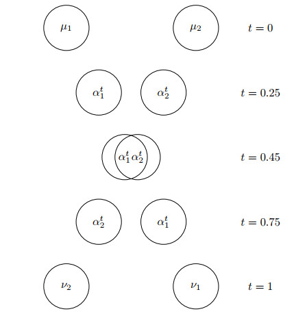
The interpolation between two opposite configurations of spheres along generalized geodesics. In particular, for $ t = 0.45 $ the pair $ (\alpha_1^t, \alpha_2^t) $ is not in $ K_2 $

The cell of the mesh in position $ (k, l) $. The densities are defined inside the cell, whereas the velocities are defined at the edges

The distribution of the image of the cell $ (2, 2) $ by T. We first compute the image of the center, then draw a box of size $ h $. The lower left part is lifted on the cell $ (3, 4) $, the upper left part on $ (3, 5) $, the upper right part on $ (4, 5) $ and the lower right part on $ (4, 4) $

Distribution of the 2-Wasserstein distances between pairs of estimated projections of the density in example 3

The motion of two crossing discs. The first column represents the sum of the two densities, and the other two the separated densities. The total time of the simulation is $ T = 0.5 $ for a timestep $ dt = 0.01 $ and a mesh size $ N = 100 $. The random projection step is averaged on $ 50 $ experiments

The motion of two crossing discs in the presence of chemoattraction. We chose the same parameters that in the previous simulation, with $ \kappa = 10 $

Aggregation of a composite crowd driven by chemoattraction and short-range interactions. For $ t = 0.50 $, we see small numerical diffusion due to the stochastic projection on $ K_2 $. The parameters here are $ N = 150 $, $ \kappa = 8 $, $ \alpha = 0.2 $, $ \eta = 0.1 $, $ R = 0.04 $. The random projection step is averaged on $ 100 $ runs and the mesh size is $ N = 150 $. The time parameters are still $ T = 0.5 $ and $ dt = 0.01 $

In solid line, the function $ g_5 $. In dashed, its approximation by a strictly convex smooth function $ f_5 $. In dotted line is displayed the common limit to $ f_n $ and $ g_n $