


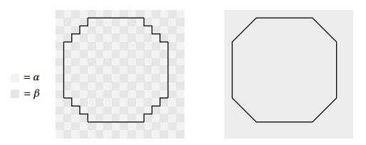
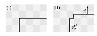
Figure 1.
Microscopic and macroscopic nontrivial equilibrium ($\alpha+\beta <0$ ).
We describe the macroscopic behavior of evolutions by crystalline curvature of planar sets in a chessboard-like medium, modeled by a periodic forcing term. We show that the underlying microstructure may produce both pinning and confinement effects on the geometric motion.
Citation: Annalisa Malusa, Matteo Novaga. Crystalline evolutions in chessboard-like microstructures[J]. Networks and Heterogeneous Media, 2018, 13(3): 493-513. doi: 10.3934/nhm.2018022
| [1] | Annalisa Malusa, Matteo Novaga . Crystalline evolutions in chessboard-like microstructures. Networks and Heterogeneous Media, 2018, 13(3): 493-513. doi: 10.3934/nhm.2018022 |
| [2] | Leonid Berlyand, Volodymyr Rybalko . Homogenized description of multiple Ginzburg-Landau vortices pinned by small holes. Networks and Heterogeneous Media, 2013, 8(1): 115-130. doi: 10.3934/nhm.2013.8.115 |
| [3] | Laura Sigalotti . Homogenization of pinning conditions on periodic networks. Networks and Heterogeneous Media, 2012, 7(3): 543-582. doi: 10.3934/nhm.2012.7.543 |
| [4] | Dimitra Antonopoulou, Georgia Karali . A nonlinear partial differential equation for the volume preserving mean curvature flow. Networks and Heterogeneous Media, 2013, 8(1): 9-22. doi: 10.3934/nhm.2013.8.9 |
| [5] | Mickaël Dos Santos, Oleksandr Misiats . Ginzburg-Landau model with small pinning domains. Networks and Heterogeneous Media, 2011, 6(4): 715-753. doi: 10.3934/nhm.2011.6.715 |
| [6] | Tasnim Fatima, Ekeoma Ijioma, Toshiyuki Ogawa, Adrian Muntean . Homogenization and dimension reduction of filtration combustion in heterogeneous thin layers. Networks and Heterogeneous Media, 2014, 9(4): 709-737. doi: 10.3934/nhm.2014.9.709 |
| [7] | Michael Helmers, Barbara Niethammer, Xiaofeng Ren . Evolution in off-critical diblock copolymer melts. Networks and Heterogeneous Media, 2008, 3(3): 615-632. doi: 10.3934/nhm.2008.3.615 |
| [8] | Hakima Bessaih, Yalchin Efendiev, Florin Maris . Homogenization of the evolution Stokes equation in a perforated domain with a stochastic Fourier boundary condition. Networks and Heterogeneous Media, 2015, 10(2): 343-367. doi: 10.3934/nhm.2015.10.343 |
| [9] | Gianni Dal Maso, Francesco Solombrino . Quasistatic evolution for Cam-Clay plasticity: The spatially homogeneous case. Networks and Heterogeneous Media, 2010, 5(1): 97-132. doi: 10.3934/nhm.2010.5.97 |
| [10] | Yilun Shang . Group pinning consensus under fixed and randomly switching topologies with acyclic partition. Networks and Heterogeneous Media, 2014, 9(3): 553-573. doi: 10.3934/nhm.2014.9.553 |
We describe the macroscopic behavior of evolutions by crystalline curvature of planar sets in a chessboard-like medium, modeled by a periodic forcing term. We show that the underlying microstructure may produce both pinning and confinement effects on the geometric motion.
We are concerned with the asymptotic behavior of motions of planar curves according to the law
| $ v = \kappa + g\left(\frac{x}{\varepsilon}, \frac{y}{\varepsilon}\right), $ | (1) |
where
Crystalline evolutions provide simplified models for describing several phenomena in Materials Science (see [25,27,28] and references therein) and have been significantly studied in recent years (see for instance [1,4,5,16,17,18,21,22]).
The forcing term
| $ F_\varepsilon(E) = \int_{\partial E} \bigl( |\nu_1^E|+|\nu_2^E|\bigr) \, d\mathcal{H}^1 +\int_E g\Bigl(\frac{x}{\varepsilon}, \frac{y}{\varepsilon}\Bigr)\ d\mathcal{L}, ~~~~ E\subset\mathbb{R}^2, $ |
where we identify the evolving curve with the boundary of a set
| $ \overline{F}(E) = \int_{\partial E} \bigl( |\nu_1^E|+|\nu_2^E|\bigr)\, d\mathcal{H}^1 +\bar g\, \mathcal{L}(E). $ |
Hence, our analysis can be set in a large class of variational evolution problems dealing with limits of motions driven by functionals
For oscillating functionals like
Coming back to our specific problem (1), we assume for simplicity that
After a careful analysis, it turns out that curves evolving by (1) undergo a microscopic "facet-breaking" phenomenon at a scale
We point out that, due to the possible presence of these new edges with zero velocity, the limit flow does not coincide with the gradient flow of the limit functional
We recall that, in a previous paper [11], we considered a similar homogenization problem where the periodic function g depends only on the horizontal variable, so that the medium has a stratified, opposite to a chessboard-like, structure.
It would be very interesting to extend our analysis to the isotropic variant of (1), where the crystalline curvature
The plan of the paper is the following: in Section 2 we introduce the notion of crystalline curvature and the evolution problem we are interested in. In Section 3 we introduce the notion of calibrable edge, that is, an edge which does not break during the evolution, and we state the calibrability conditions. Finally, in Section 4 we characterize explicitly the limit evolution as
Notation.The canonical basis of
The 1-dimensional Hausdorff measure and the 2-dimensional Lebesgue measure in
We say that a set
The Hausdorff distance between two sets
The crystalline curvature.We briefly recall a notion of curvature
| $ P_\varphi(E): = \int_{\partial E} \bigl(|\nu_1^E|+|\nu_2^E|\bigr)\, d\mathcal{H}^1, $ |
has normal velocity
The surface tension
Given a nonempty compact set
| $ d^E(\xi): = \inf\limits_{\eta\in E}\varphi(\xi-\eta) - \inf\limits_{\eta\not\in E}\varphi(\xi-\eta), ~~~~ \xi\in\mathbb{R}^2. $ |
The normal cone at
| $ T_{\varphi^\circ}(\xi^\circ) : = \{\xi\in \mathbb{R}^2, \ \xi\cdot\xi^\circ = (\varphi^\circ(\xi))^2\}, ~~~~\xi^\circ\in\mathbb{R}^2\, . $ |
The notion of intrinsic curvature in
Definition 2.1 (
Any selection of the multivalued function
Remark 1 (Edges and vertices). A direct computation gives that
|
$
{Tφ∘(e1)=[[(1,1),(1,−1)]],Tφ∘(e2)=[[(−1,1),(1,1)]],Tφ∘(−e1)=[[(−1,1),(−1,−1)]],Tφ∘(−e2)=[[(−1,−1),(1,−1)]].
$
|
(Here and in the following
The requirement of Lipschitz continuity keeps the value of every Cahn-Hoffmann vector field fixed at vertices. Hence, in order to exhibit a Cahn-Hoffmann vector field
Forced crystalline flows. Let
|
$
g(x, y) = {α,in ]0,12[2⋃]12,1[2,β,in (]12,1[×]0,12[)⋃(]0,12[×]12,1[),
$
|
(2) |
and extended by periodicity in
We will denote by
We define the multifunction
We want to introduce our notion of geometric evolution
| $ v = \kappa+g_\varepsilon, ~~~~\text{on}\ \partial E, $ | (3) |
where
In order to give a meaning to (3) it would be enough to require that the evolution is a family of
This ambiguity can be overcome introducing an additional postulate, which is consistent with the notion of forced curve shortening flow (see [4], [5], [6], [23], [24]).
Definition 2.2 (Variational Cahn-Hoffmann field). A variational Cahn-Hoffmann vector field for a
| $ \mathcal{N}_{L}(n) = \int_{L} |g_\varepsilon +{\rm{div}} n|^2\, d\mathcal{H}^1 $ |
in the set
| $ D_L = \left\{ n \in L^\infty(L, \mathbb{R}^2), n\in T_{L}, {\rm{div}} n\in L^\infty(L), n(p) = n_0, n(q) = n_1 \right\} $ |
where
Remark 2. If the minimum
| $ \kappa^{L} = \chi_{L}\frac{2}{\ell} \ \text{on}\ L, $ |
where
Definition 2.3 (Forced crystalline evolution). Given
(ⅰ)
(ⅱ) there exists an open set
(ⅲ) there exists a function
(ⅳ)
In this section we deal with the minimum problem in Definition 2.2 for a given
The results concern edges
Setting by
|
$
(BV) = {n(p)=n(q)=n0∈{±1}if χL=0;n(p)=−1, n(q)=1,if χL=1;n(p)=1, n(q)=−1,if χL=−1.
$
|
(4) |
Moreover, we denote by
| $ \mathcal{I}_{\beta, \alpha} = \{s\in \mathbb{R} \colon\ \gamma_\varepsilon = \alpha\ \text{in} \ ]s, s+\varepsilon /2[\}, ~~~~ \mathcal{I}_{\alpha, \beta} = \{s\in \mathbb{R} \colon\ \gamma_\varepsilon = \beta\ \text{in} \ ]s, s+\varepsilon /2[\}. $ |
With this notation, the requirement that
Definition 3.1 (Calibrability conditions).
(ⅰ)
(ⅱ)
(ⅲ)
In this case, we say that
The calibrability property was studied, in its full generality, in [11]. We collect here the results needed in the rest of the paper, sketching the proofs for sake of completeness.
Denoting by
| $ \ell - \varepsilon\left\lfloor\dfrac{\ell}{\varepsilon}\right\rfloor = \ell_{\alpha}+ \ell_{\beta}, ~~~~ \int_L \gamma_\varepsilon(s)\, ds = \frac{\alpha+\beta}{2}\left(\ell- \ell_{\alpha}-\ell_{\beta}\right)+\alpha \ell_{\alpha}+\beta \ell_{\beta}, $ | (5) |
the calibrability condition in Definition 3.1(ⅲ) sets the value of
|
$
n'(s) = {12ℓ(4χL+(β−α)(ℓ−ℓα+ℓβ))if γε(s)=α,12ℓ(4χL−(β−α)(ℓ+ℓα−ℓβ)),if γε(s)=β.
$
|
(6) |
so that
| $ n(s) = n(p)+(s-p)v_L-\int_p^s \gamma_\varepsilon(\tau)\, d\tau, $ | (7) |
where
| $ \label{f:velocita} v_L = \chi_L\frac{2}{\ell}+\frac{\alpha+\beta}{2}+ \frac{\beta-\alpha}{2\ell}(\ell_\beta -\ell_\alpha). $ | (8) |
In conclusion, the calibrability conditions (ⅰ) and (ⅲ) in Definition 3.1 fix a candidate field (7) which is continuous and affine with given slope in each phase of
Remark 3. In what follows we will assume
Proposition 3.2. Let
(i) If
(ia)
(ib)
(ii) If
(iia)
(iib)
Proof. If
If
| $ n(p+\varepsilon)-n(p) = \frac{\varepsilon}{2\ell}(\beta-\alpha) (\ell_\beta-\ell_\alpha) = n(q)-n(q-\varepsilon), $ |
and hence, since
|
$
n'(x) = {β−α2if γε(x)=α,α−β2if γε(x)=β,
$
|
and a Canh-Hoffmann vector field with this derivative exists only if
The case
Proposition 3.3. Let
| $ \ell+\ell_\alpha-\ell_\beta \leq \frac{4}{\beta-\alpha} $ | (9) |
or
Proof. Under the assumption (9), the candidate Cahn-Hoffmann vector field (7) is an increasing function in
Assume now that
| $ n(p+\varepsilon)-n(p) = \frac{\varepsilon}{4\ell} \left(8-(\beta-\alpha)\varepsilon\right) > 0. $ |
Similarly, we obtain that
Remark 4. Notice that, if
| $ v_L\geq \frac{2}{\ell}+\frac{\alpha+\beta}{2}+ +\frac{\beta-\alpha}{2\ell} \left(\ell-\frac{4}{\beta-\alpha}\right) = \beta > 0 $ |
Proposition 3.4. Let
(i) If either
(ii) If
| $ m = \varepsilon \frac{\beta-\alpha}{(\beta-\alpha)(\tilde{\ell}+\varepsilon/2)+4}, ~~~~ h = \frac{\varepsilon}{2}\frac{(\beta-\alpha)(\tilde{\ell}+\varepsilon/2)-4} {(\beta-\alpha)(\tilde{\ell}+\varepsilon/2)+4}, $ |
and
| $ \Sigma = \left\{m\sigma_2 +h \leq \sigma_1 \leq \frac{1}{m} \sigma_2- \frac{h}{m}\right\}, $ |
we have
| $ v_L = \frac{2}{\ell}+\frac{\alpha+\beta}{2}+\frac{\beta-\alpha}{2\ell} \left(\frac{\varepsilon}{2}-\sigma_1-\sigma_2\right) $ |
if and only if
(iii) if
| $ \sigma^* = \frac{\varepsilon}{2}\frac{(\beta-\alpha)(\ell^*+\varepsilon/2)-4} {(\beta-\alpha)(\ell^*-\varepsilon/2)+4}. $ |
Then
Proof. If
If both the endpoints belong to the
|
$
{n(p+ε/2+σ1)−n(p)≥0,n(q−ε/2−σ2)−n(q)≥0
$
|
that guarantee the calibrability of the edge.
Setting
| $ \tilde{\sigma}: = \frac{\varepsilon}{2}\frac{(\beta-\alpha)(\tilde{\ell}+\varepsilon/2)-4} {(\beta-\alpha)(\tilde{\ell}-\varepsilon/2)+4}, $ | (10) |
we have that
The proof of (ⅲ) follows by the same arguments.
Remark 5 (Calibrability threshold). In the special case when
Similarly, in the case of Proposition 3.4(ⅲ), when
The results of Section 3 prescribe a velocity to every calibrable edge not lying on a discontinuity line of
In every time interval between these events, the motion is determined by a system of ODEs, and hence the behavior of the evolution on the discontinuities can be described using the general theory of differential equations with discontinuous right-hand side [20].
Concerning the changes of geometry, it is clear what is meant by "disappearing edges", that is edges whose length becomes zero in finite time, but the notion of "appearing edges", that is how a no longer calibrable edge breaks, has to be specified.
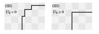
We focus our attention to coordinate polyrectangles whose edges have non-negative
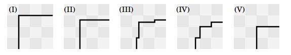
Definition 4.1 (Cracking multiplicity and set-up). If
| $ L^c: = \sup \{\tilde{L}\subseteq L\colon \ \tilde{L} = [s_1, s_2], \ n(s_1) = n(p), n(s_2) = n(q), \ \tilde{L} \ \text{calibrable}\} = [p_b, q_b], $ |
and let us denote by
|
$
M(L): = {1,if L=Lc,3,if L≠Lc, and either L−=∅, or L+=∅, 5,if L−≠∅, and L+≠∅.
$
|
The points
For every edge
| $ v^{in}_L = \chi_{L}\frac{2}{\ell}+ \frac{1}{\ell} \int_{L+\frac{\varepsilon }{4}\nu(L)} g_\varepsilon , ~~~~ v^{out}_L = \chi_{L}\frac{2}{\ell}+ \frac{1}{\ell} \int_{L-\frac{\varepsilon }{4}\nu(L)} g_\varepsilon . $ | (11) |
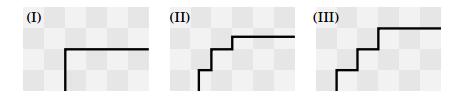
If
|
$
M(L) = {M(L+ε4ν(L))if vinL>0 and voutL≥0M(L−ε4ν(L))if vinL≤0 and voutL<01if vinL≤0 and voutL≥0
$
|
When
Proposition 4.2. Let
(i)
(ii)
(iii)
Proof. Let
| $ p_b = \min\{s\in [p, q]\cap \mathcal{I}_{\beta, \alpha}\}, ~~~~ q_b = \max\{s\in [p, q]\cap \mathcal{I}_{\alpha, \beta}\}, $ |
Moreover, by Proposition 3.2,
Concerning the velocities, assume that
| $ v^- = v(\sigma) = \frac{ \sigma \alpha +\frac{\varepsilon }{2} \beta}{ \sigma +\frac{\varepsilon }{2}} $ |
with
Recalling Proposition 3.2, we can perform a similar splitting for edges with zero
| $ p_b = \min\{s\in [p, q]\cap \mathcal{I}_{\alpha, \beta}\}, ~~~~ q_b = \max\{s\in [p, q]\cap \mathcal{I}_{\alpha, \beta}\}, $ |
while, if
| $ p_b = \min\{s\in [p, q]\cap \mathcal{I}_{\beta, \alpha}\}, ~~~~ q_b = \max\{s\in [p, q]\cap \mathcal{I}_{\beta, \alpha}\}. $ |
In both cases the remaining parts
| $ v^\pm = \frac{\sigma_\alpha^\pm \alpha+\sigma_\beta^\pm \beta}{\sigma_\alpha^\pm +\sigma_\beta^\pm }, $ |
for suitable
The case of
Definition 4.3 (Breaking configuration). Let
Remark 6. By Proposition 4.2, a breaking configuration of the boundary of a coordinate polyrectagle
The following result shows that, in our setting, the evolution is well posed.
Proposition 4.4. Let
(1)
(2)
(3)
then the evolution is unique. Moreover if
Proof. A given coordinate polyrectangle
Let us denote
We associate to
If
By Definition 2.3, a forced crystalline flow
| $ s' = V(s) ~~~~\text{in}\ [0, T] $ | (12) |
where
| $ \Sigma = \left\{s\in \mathbb{R}^m \colon \ \exists s_i\in \frac{\varepsilon }{2}\mathbb{Z}\right\}, $ |
and defined outside
| $ V = (V_1, \ldots, V_m), \ V_i(s) = -\left(\chi_{L_i}\frac{2}{\ell_i(s)}+ \frac{1}{\ell_i(s)} \int_{L_i(s)} g_\varepsilon \right), \ i = 1, \ldots, m, \ s\not\in \Sigma. $ |
Notice that the fictitious edges with zero length, possibly added in the breaking configuration of
System (12) fits therefore into Filippov's theory of discontinuous dynamical systems (see [20], [19]): the field
| $ F(V)(s) = \text{co}\left\{\lim\limits_{k\to \infty}V(s^k), s^k \to s, \ s_k \not\in \Sigma \right\}, ~~~~s \in\Sigma, $ | (13) |
(where we denote by
In order to deal with the uniqueness of solutions, we need an explicit computation of the multifunction
For every
|
$
V+i(s)=−(χLi2ℓi(s)+1ℓi(s)∫Li(s)+ε4νigε),V−i(s)=−(χLi2ℓi(s)+1ℓi(s)∫Li(s)−ε4νigε),
$
|
and let
For every
| $ F(V)(s) = I_1(s) \times \cdots \times I_m(s) $ |
where
|
$
I_i(s) = {{Vi(s)},if si∉ε2Z,I(V−i(s),V+i(s))if si∈ε2Z,and ℓi>0[α,β]if si∈ε2Z,and ℓi=0, ~~~~
i = 1, \ldots, m.
$
|
Assume now that every element of the breaking configuration of
Concerning the edges with zero length, notice that if
Let
Then, for every
On the other hand, for every
In conclusion, since the function
|
$
s'_i = {0i∈N1Vi(s)i∈N2∪N3. ~~~~
\text{a.e. in} \ ]0, \overline{t}[.
$
|
In terms of the breaking configuration of
Remark 7. As a consequence of Proposition 4.4, if
(a) every vertex of
(b) every edge of
(c) every edge of
is pinned. Namely, requirement (a) implies that every edge of
| $ v^{in}_L = \frac{2}{\ell} +\frac{\alpha+\beta}{2}- \frac{(\beta-\alpha)\varepsilon}{4 \ell} < 0, ~~~~ v^{out}_L = \frac{2}{\ell} +\frac{\alpha+\beta}{2}+ \frac{(\beta-\alpha)\varepsilon}{4 \ell} > 0. $ |
for every edge
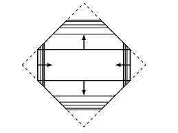
In particular, the symmetric equilibria
In conclusion, the forced crystalline evolutions defined in Definition 2.3 and starting from a polyrectangle are obtained by the following procedure: we set-up the initial datum and we obtain the evolution
We are interested in stressing the macroscopic effect of the underling periodic structure on the geometric evolutions, depicting clearly the forced crystalline flows and passing to the limit as
In what follows
Theorem 4.5 (Effective motion of coordinate squares). Let
(i) If either
|
$
{ℓ′=−4ℓ−(α+β),ℓ(0)=ℓ0,
$
|
(14) |
and then shrinking to a point in finite time.
(ii) If
|
$
{ℓ′=4ℓ+(α+β),ℓ(0)=ℓ0,
$
|
(15) |
and then
Proof. Given
Case (ia):
By Proposition 3.3, the breaking configuration of
| $ {(\ell^\varepsilon )}' = -\frac{4}{\ell^\varepsilon }-(\alpha+\beta)- \frac{\beta-\alpha}{\ell^\varepsilon }(\ell_\beta^\varepsilon -\ell_\alpha^\varepsilon ). $ | (16) |
Since
Case (ib): either
As a first step, we assume, in addition, that every vertex of
| $ M(L^\varepsilon ) = M\left(L^\varepsilon + \frac{\varepsilon }{4}\nu(L^\varepsilon )\right) = 1, ~~~~ \forall L^\varepsilon \subseteq \partial S(\ell_0^\varepsilon ), $ |
and, by Proposition 4.4, there exists a unique forced crystalline flow starting from
| $ t_0 = \sup\{t > 0 \colon \ S(\ell(s))\ \text{is calibrable for every}\ s \in ]0, t[\} $ |
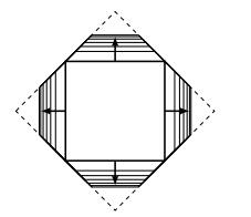
(see Figure 2(Ⅱ)). By symmetry, the breaking set-up of every edge of
| $ \frac{\varepsilon }{2}+\tilde{\sigma} = |p_i-p_{i, b}| = |q_i-q_{i, b}| = |p_j-p_{j, b}| = |q_j-q_{j, b}|~~~~ \forall i, j = 1, \ldots, 4, $ |
where
Then, by Proposition 4.4, the evolution admits a unique extension
| $ v_c^\varepsilon = \frac{2}{\ell_0^\varepsilon -2\varepsilon }+\frac{\alpha+\beta}{2}+ \frac{(\alpha-\beta)\varepsilon}{4(\ell_0^\varepsilon -2 \varepsilon )}, $ | (17) |
while the small edges with zero
| $ \varepsilon > v_c^\varepsilon (t_2-t_1) > (k+o(\varepsilon ))(t_2-t_1), $ |
where
Since
Moreover, for every square
Case (ⅱ):
If every vertex of
| $ M(L^\varepsilon ) = M\left(L^\varepsilon - \frac{\varepsilon }{4}\nu(L^\varepsilon )\right) = 5, ~~~~ \forall L^\varepsilon \subseteq \partial S(\ell_0^\varepsilon ), $ |
and, by Proposition 4.2, every edge of
Then the process iterates, "cutting" the square and reducing the length
| $ v^\varepsilon (t) = \frac{2}{\ell^\varepsilon (t)} +\frac{\alpha+\beta}{2}- \frac{(\beta-\alpha)\varepsilon}{4 \ell^\varepsilon (t)}, $ |
until the first time
Finally, notice that the forced crystalline evolution starting from a general initial datum
The arguments used in the proof of Theorem 4.5 can be applied to deal with every polyrectangle (and hence, by approximation, to describe the effective evolution of general sets), but a detailed analysis of the forced crystalline flow in these cases requires considerable additional computations. Just to appreciate the application of the previous arguments in a slightly more general setting, we devote the end of this section to a coincise description of the motion starting from coordinate rectangles.
In what follows
Theorem 4.6 (Effective motion of coordinate rectangles). Let
| $ v_{i, 0}: = \frac{2}{\ell_{i, 0}} +\frac{\alpha+\beta}{2}, ~~~~i = 1, 2 $ |
in the following way.
(i) If
|
$
{ℓ′1=−4ℓ2−(α+β),ℓ′2=−4ℓ1−(α+β),ℓ1(0)=ℓ1,0,ℓ2(0)=ℓ2,0.
$
|
(18) |
(ii) If either
|
$
{ℓ′1=4ℓ1+(α+β),ℓ′2=4ℓ2+(α+β),ℓ1(0)=ℓ1,0,ℓ2(0)=ℓ2,0.
$
|
(19) |
(iii) If
Proof. When either
Assume that every vertex of the approximating initial datum
| $ M(L^\varepsilon _1) = M\left(L^\varepsilon _1-\frac{\varepsilon }{4}\nu(L^\varepsilon _1)\right) = 3, $ |
while
| $ M(L^\varepsilon _2) = M\left(L^\varepsilon _2+\frac{\varepsilon }{4}\nu(L^\varepsilon _2)\right) = 1. $ |
Therefore the forced evolution starts breaking the edge
Setting
| $ U(\ell_1, \ell_2): = \frac{1}{\ell_{1}}+\frac{1}{\ell_{2}} +\frac{\alpha+\beta}{2}, $ | (20) |
the subsequent evolution depends on the sign of
If
| $ v_i^\varepsilon (t) = \frac{2}{\ell_i^\varepsilon (t)} +\frac{\alpha+\beta}{2}- \frac{(\beta-\alpha)\varepsilon}{4 \ell_i^\varepsilon (t)}, ~~~~ i = 1, 2. $ |
Then, the effective evolution
If
If
|
$
{(ℓε1)′=−2(2ℓε2+α+β2−(β−α)ε4ℓε2),(ℓε2)′=−2(2ℓε1+α+β2−(β−α)ε4ℓε1).
$
|
Passing to the limit as
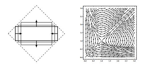
| $ A: = \{U(\ell_1, \ell_2) > 0\}\cap \left\{\ell_2\leq \frac{-4}{\alpha+\beta} \leq \ell_1\right\}. $ |
Notice that the function
| $ J(\ell_1, \ell_2) = 4(\log (\ell_2) - \log (\ell_1))+ (\alpha+\beta) (\ell_2-\ell_1) $ |
is a constant of motion for system (18). The phase portrait is shown in Figure 8. In particular,
The level set
If
If
The geometric evolution in Definition 2.3 provides a possible mathematical model for the interface motion in a variety of material science problems. Our setting fits, for example, with the description of growth (or dissolution) of a crystal, whose structure manifests itself in the dependency of the interfacial energy density
In previous papers [1,3,22] the assumption that every facet of the crystal moves parallely to itself during the evolution facilitates the description of the motion, and leads to a system of ODEs satisfied by the lengths of the facets.
In our model the underlying microstructure is oscillating between two phases
Our results shows that, in this simple setting, the effective motion of the interface, obtained as a limit as
The authors wish to thank Andrea Braides for useful discussions on the topic of this paper. The second author was partially supported by the Italian CNR-GNAMPA and by the University of Pisa via grant PRA-2017 "Problemi di ottimizzazione e di evoluzione in ambito variazionale".
| [1] |
Flat flow is motion by crystalline curvature for curves with crystalline energies. J. Differential Geometry (1995) 42: 1-22. 
|
| [2] |
Homogenization of fronts in highly heterogeneous media. SIAM J. Math. Anal. (2011) 43: 212-227.
|
| [3] | Approximation to driven motion by crystalline curvature in two dimensions. Adv. Math. Sci. and Appl. (2000) 10: 467-493. |
| [4] |
Characterization of facet breaking for nonsmooth mean curvature flow in the convex case. Interfaces Free Bound. (2001) 3: 415-446.
|
| [5] |
On a crystalline variational problem, part Ⅰ: First variation and global $L^∞$ regularity. Arch. Rational Mech. Anal (2001) 57: 165-191.
|
| [6] |
On a crystalline variational problem, part Ⅱ: $BV$ regularity and structure of minimizers on facets. Arch. Rational Mech. Anal. (2001) 157: 193-217.
|
| [7] |
A. Braides,
$Γ$-convergence for Beginners, Oxford University Press, 2002. doi: 10.1093/acprof:oso/9780198507840.001.0001
|
| [8] |
A. Braides, Local Minimization, Variational Evolution and Γ–convergence, Lecture Notes in
Mathematics, Springer, Berlin, 2014. doi: 10.1007/978-3-319-01982-6
|
| [9] |
Crystalline Motion of Interfaces Between Patterns. J. Stat. Phys. (2016) 165: 274-319.
|
| [10] |
Motion and pinning of discrete interfaces. Arch. Ration. Mech. Anal. (2010) 195: 469-498.
|
| [11] |
A. Braides, A. Malusa and M. Novaga, Crystalline evolutions with rapidly oscillating forcing
terms, to appear on Ann. Scuola Norm. Sci. doi: 10.2422/2036-2145.201707_011
|
| [12] |
Motion of discrete interfaces in periodic media. Interfaces Free Bound. (2013) 15: 451-476.
|
| [13] |
Motion of discrete interfaces through mushy layers. J. Nonlinear Sci. (2016) 26: 1031-1053.
|
| [14] |
Homogenization of a semilinear heat equation. J. Éc. polytech. Math. (2017) 4: 633-660.
|
| [15] |
Curve shortening flow in heterogeneous media. Interfaces and Free Bound. (2011) 13: 485-505.
|
| [16] |
Existence and uniqueness for a crystalline mean curvature flow. Comm. Pure Appl. Math. (2017) 70: 1084-1114.
|
| [17] | A. Chambolle, M. Morini, M. Novaga and M. Ponsiglione, Existence and uniqueness for anisotropic and crystalline mean curvature flows, preprint, arXiv: 1702.03094. |
| [18] |
Approximation of the anisotropic mean curvature flow. Math. Models Methods Appl. Sci. (2007) 17: 833-844.
|
| [19] |
Discontinuous Dynamical Systems: A tutorial on solutions, nonsmooth analysis, and stability. IEEE Control Systems Magazine (2008) 28: 36-73.
|
| [20] |
A. F. Filippov,
Differential Equations with Discontinuous Righthand Sides, vol. 18 of Mathematics and Its Applications. Dordrecht, The Netherlands, Kluwer Academic Publishers, 1988. doi: 10.1007/978-94-015-7793-9
|
| [21] | Y. Giga, Surface Evolution Equations. A Level Set Approach, vol. 99 of Monographs in Mathematics. Birkhäuser Verlag, Basel, 2006. |
| [22] |
A comparison theorem for crystalline evolution in the plane. Quarterly of Applied Mathematics (1996) 54: 727-737.
|
| [23] |
Facet bending in the driven crystalline curvature flow in the plane. J. Geom. Anal. (2008) 18: 109-147.
|
| [24] |
Facet bending driven by the planar crystalline curvature with a generic nonuniform forcing term. J. Differential Equations (2009) 246: 2264-2303.
|
| [25] | M. E. Gurtin, Thermomechanics of Evolving Phase Boundaries in the Plane, Oxford Mathematical Monographs. The Clarendon Press, Oxford University Press, New York, 1993. |
| [26] |
Closed curves of prescribed curvature and a pinning effect. Netw. Heterog. Media (2011) 6: 77-88.
|
| [27] |
Crystalline variational problems. Bull. Amer. Math. Soc. (1978) 84: 568-588.
|
| [28] | Geometric Models of Crystal Growth. Acta Metall. Mater. (1992) 40: 1443-1474. |
| 1. | Giovanni Scilla, Motion of Discrete Interfaces on the Triangular Lattice, 2020, 88, 1424-9286, 315, 10.1007/s00032-020-00316-5 | |
| 2. | Andrea Braides, Margherita Solci, 2021, Chapter 4, 978-3-030-69916-1, 53, 10.1007/978-3-030-69917-8_4 |
Annalisa Malusa, Matteo Novaga. Crystalline evolutions in chessboard-like microstructures[J]. Networks and Heterogeneous Media, 2018, 13(3): 493-513. doi: 10.3934/nhm.2018022

 DownLoad:
