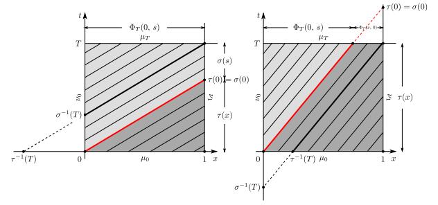
In this paper we formulate a theory of measure-valued linear transport equations on networks. The building block of our approach is the initial and boundary-value problem for the measure-valued linear transport equation on a bounded interval, which is the prototype of an arc of the network. For this problem we give an explicit representation formula of the solution, which also considers the total mass flowing out of the interval. Then we construct the global solution on the network by gluing all the measure-valued solutions on the arcs by means of appropriate distribution rules at the vertexes. The measure-valued approach makes our framework suitable to deal with multiscale flows on networks, with the microscopic and macroscopic phases represented by Lebesgue-singular and Lebesgue-absolutely continuous measures, respectively, in time and space.
Citation: Fabio Camilli, Raul De Maio, Andrea Tosin. Transport of measures on networks[J]. Networks and Heterogeneous Media, 2017, 12(2): 191-215. doi: 10.3934/nhm.2017008
In this paper we formulate a theory of measure-valued linear transport equations on networks. The building block of our approach is the initial and boundary-value problem for the measure-valued linear transport equation on a bounded interval, which is the prototype of an arc of the network. For this problem we give an explicit representation formula of the solution, which also considers the total mass flowing out of the interval. Then we construct the global solution on the network by gluing all the measure-valued solutions on the arcs by means of appropriate distribution rules at the vertexes. The measure-valued approach makes our framework suitable to deal with multiscale flows on networks, with the microscopic and macroscopic phases represented by Lebesgue-singular and Lebesgue-absolutely continuous measures, respectively, in time and space.

| [1] | L. Ambrosio, N. Gigli and G. Savaré, Gradient Flows in Metric Spaces and in the Space of Probability Measures, Lectures in Mathematics ETH Zürich, Birkhäuser Verlag, Basel, 2008. |
| [2] |
(2007) Measure Theory. Berlin Heidelberg: Springer-Verlag. 
|
| [3] |
An easy-to-use algorithm for simulating traffic flow on networks: Numerical experiments. Discrete Contin. Dyn. Syst. Ser. S (2014) 7: 379-394.
|
| [4] |
An easy-to-use algorithm for simulating traffic flow on networks: Theoretical study. Netw. Heterog. Media (2014) 9: 519-552.
|
| [5] |
Stationary mean field games systems defined on networks. SIAM J. Control. Optim. (2016) 54: 1085-1103.
|
| [6] |
A well-posedness theory in measures for some kinetic models of collective motion. Math. Models Methods Appl. Sci. (2011) 21: 515-539.
|
| [7] |
E. Cristiani, B. Piccoli and A. Tosin,
Multiscale Modeling of Pedestrian Dynamics, vol. 12 of MS & A: Modeling, Simulation and Applications, Springer International Publishing, 2014. doi: 10.1007/978-3-319-06620-2
|
| [8] |
On the micro-to-macro limit for first-order traffic flow models on networks. Netw. Heterog. Media (2016) 11: 395-413.
|
| [9] |
Modelling supply networks with partial differential equations. Quart. Appl. Math. (2009) 67: 419-440.
|
| [10] |
Vertex control of flows in networks. Netw. Heterog. Media (2008) 3: 709-722.
|
| [11] |
Mild solutions to a measure-valued mass evolution problem with flux boundary conditions. J. Differential Equations (2015) 259: 1068-1097.
|
| [12] |
Measure-valued mass evolution problems with flux boundary conditions and solution-dependent velocities. SIAM J. Math. Anal. (2016) 48: 1929-1953.
|
| [13] |
A fully-discrete-state kinetic theory approach to traffic flow on road networks. Math. Models Methods Appl. Sci. (2015) 25: 423-461.
|
| [14] | M. Garavello and B. Piccoli, Traffic Flow on Networks -Conservation Laws Models, AIMS Series on Applied Mathematics, American Institute of Mathematical Sciences, Springfield, MO, 2006. |
| [15] |
Models of discrete and continuous cell differentiation in the framework of transport equation. SIAM J. Math. Anal. (2012) 44: 1103-1133.
|
| [16] |
D. Mugnolo,
Semigroup Methods for Evolution Equations on Networks, Understanding Complex Systems, Springer International Publishing, 2014. doi: 10.1007/978-3-319-04621-1
|
| [17] |
Generalized Wasserstein distance and its application to transport equations with source. Arch. Ration. Mech. Anal. (2014) 211: 335-358.
|
| [18] |
Differential equations on networks. J. Math. Sci. (N. Y.) (2004) 119: 691-718.
|
| [19] | D. T. H. Worm, Semigroups on Spaces of Measures, PhD thesis, Leiden University, 2010. |


Figures(3)
Fabio Camilli, Raul De Maio, Andrea Tosin. Transport of measures on networks[J]. Networks and Heterogeneous Media, 2017, 12(2): 191-215. doi: 10.3934/nhm.2017008


 DownLoad: