Fractional modeling of COVID-19 pandemic model with real data from Pakistan under the ABC operator

Rahat Zarin; Amir Khan; Aurangzeb; Ali Akgül; Esra Karatas Akgül; Usa Wannasingha Humphries; Rahat Zarin; Amir Khan; Aurangzeb; Ali Akgül; Esra Karatas Akgül; Usa Wannasingha Humphries

doi:10.3934/math.2022872

AIMS Mathematics

2022, Volume 7, Issue 9: 15939-15964. doi: 10.3934/math.2022872

Previous Article Next Article

Research article Special Issues

Fractional modeling of COVID-19 pandemic model with real data from Pakistan under the ABC operator

1.
Department of Basic Sciences, University of Engineering and Technology Peshawar, Khyber Pakhtunkhwa, Pakistan
2.
Department of Mathematics and Statistics, University of Swat, Khyber Pakhtunkhawa, Pakistan
3.
Department of Mathematics, Faculty of Science, King Mongkut's University of Technology Thonburi (KMUTT), 126 Pracha-Uthit Road, Bang Mod, Thrung Khru, Bangkok 10140, Thailand
4.
Siirt University, Art and Science Faculty of Science, Department of Mathematics, TR-56100 Siirt, Turkey

Received: 27 February 2022 Revised: 18 April 2022 Accepted: 27 April 2022 Published: 28 June 2022
MSC : 37G05, 37G15, 39A28, 92B05

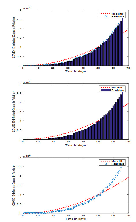
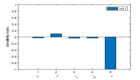
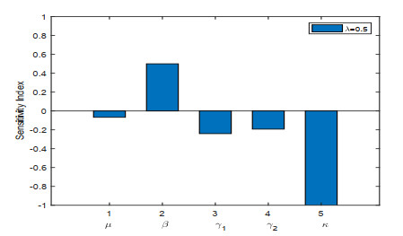
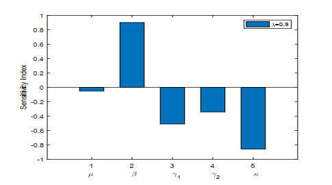
In this study, the COVID-19 epidemic model is established by incorporating quarantine and isolation compartments with Mittag-Leffler kernel. The existence and uniqueness of the solutions for the proposed fractional model are obtained. The basic reproduction number, equilibrium points, and stability analysis of the COVID-19 model are derived. Sensitivity analysis is carried out to elaborate the influential parameters upon basic reproduction number. It is obtained that the disease transmission parameter is the most dominant parameter upon basic reproduction number. A convergent iterative scheme is taken into account to simulate the dynamical behavior of the system. We estimate the values of variables with the help of the least square curve fitting tool for the COVID-19 cases in Pakistan from 04 March to May 10, 2020, by using MATLAB.
- real data,
- pandemic model,
- stability analysis,
- sensitivity analysis,
- numerical simulations
Citation: Rahat Zarin, Amir Khan, Aurangzeb, Ali Akgül, Esra Karatas Akgül, Usa Wannasingha Humphries. Fractional modeling of COVID-19 pandemic model with real data from Pakistan under the ABC operator[J]. AIMS Mathematics, 2022, 7(9): 15939-15964. doi: 10.3934/math.2022872

Related Papers:

Abstract

In this study, the COVID-19 epidemic model is established by incorporating quarantine and isolation compartments with Mittag-Leffler kernel. The existence and uniqueness of the solutions for the proposed fractional model are obtained. The basic reproduction number, equilibrium points, and stability analysis of the COVID-19 model are derived. Sensitivity analysis is carried out to elaborate the influential parameters upon basic reproduction number. It is obtained that the disease transmission parameter is the most dominant parameter upon basic reproduction number. A convergent iterative scheme is taken into account to simulate the dynamical behavior of the system. We estimate the values of variables with the help of the least square curve fitting tool for the COVID-19 cases in Pakistan from 04 March to May 10, 2020, by using MATLAB.

References

[1]	J. Wang, R. Zhang, T. Kuniya, The stability anaylsis of an SVEIR model with continuous age-structure in the exposed and infection classes, J. Biol. Dynam., 9 (2015), 73–101. https://doi.org/10.1080/17513758.2015.1006696 doi: 10.1080/17513758.2015.1006696
[2]	G. Hussain, T. Khan, A. Khan, M. Inc, G. Zaman, K. S. Nisar, et al. Modeling the dynamics of novel coronavirus (COVID-19) via stochastic epidemic model, Alex. Eng. J., 60 (2021), 4121–4130. https://doi.org/10.1016/j.aej.2021.02.036 doi: 10.1016/j.aej.2021.02.036
[3]	M. A. Khan, The dynamics of dengue infection through fractal-fractional operator with real statistical data, Alex. Eng. J., 60 (2021), 321–336. https://doi.org/10.1016/j.aej.2020.08.018 doi: 10.1016/j.aej.2020.08.018
[4]	Z. Gul, Y. H. Kang, I. H. Jung, Stability analysis and optimal vaccination of an SIR epidemic model, Biosystems, 93 (2008), 240–249. https://doi.org/10.1016/j.biosystems.2008.05.004 doi: 10.1016/j.biosystems.2008.05.004
[5]	A. A. Mohsen, H. F. Al-Husseiny, X. Zhou, K. Hattaf, Global stability of COVID-19 model involving the quarantine strategy and media coverage effects, AIMS public Health, 7 (2020), 587–605. https://doi.org/10.3934/publichealth.2020047 doi: 10.3934/publichealth.2020047
[6]	T. N. Huy, H. Mohammadi, S. Rezapour, A mathematical model for COVID-19 transmission by using the Caputo fractional derivative, Chaos Soliton. Fract., 140 (2020), 110107. https://doi.org/10.1016/j.chaos.2020.110107 doi: 10.1016/j.chaos.2020.110107
[7]	Z. Liu, H. Shao, D. Alahmadi, Numerical calculation and study of differential equations of muscle movement velocity based on martial articulation body ligament tension, Appl. Math. Nonlinear Sci., 2021. https://doi.org/10.2478/amns.2021.1.00051
[8]	Y. Zhao, A. Khan, U. W Humphries, R. Zarin, M. Khan, A. Yusuf, Dynamics of Visceral Leishmania Epidemic Model with Non-Singular Kernel, Fractals, 2022. https://doi.org/10.1142/S0218348X22401351
[9]	W. Beibei, A. Al-Barakati, H. Hasan, Characteristics of mathematical statistics model of student emotion in college physical education, Appl. Math. Nonlinear Sci., 2021. https://doi.org/10.2478/amns.2021.2.00023
[10]	J. Zhou, L. Li, Z. Yu, The transfer of stylised artistic images in eye movement experiments based on fuzzy differential equations, Appl. Math. Nonlinear Sci., 2021. https://doi.org/10.2478/amns.2021.1.00048
[11]	L. Yali, C. Chen, R. Alotaibi, S. M. Shorman, Study on audio-visual family restoration of children with mental disorders based on the mathematical model of fuzzy comprehensive evaluation of differential equation, Appl. Math. Nonlinear Sci., 2021. https://doi.org/10.2478/amns.2021.1.00090
[12]	A. Khan, R. Zarin, G. Hussain, A. H. Usman, U. W. Humphries, J. F. Gomez-Aguilard, Modeling and sensitivity analysis of HBV epidemic model with convex incidence rate, Results Phys., 22 (2021), 103836. https://doi.org/10.1016/j.rinp.2021.103836 doi: 10.1016/j.rinp.2021.103836
[13]	X. Li, X. Yang, K. H. Alyoubi, R. E. Omer, Educational research on mathematics differential equation to simulate the model of children's mental health prevention and control system, Appl. Math. Nonlinear Sci., 2021. https://doi.org/10.2478/amns.2021.2.00068
[14]	Z. Licong, F. S. Alotaibi, College students' mental health climbing consumption model based on nonlinear differential equations, Appl. Math. Nonlinear Sci., 2021. https://doi.org/10.2478/amns.2021.2.00080
[15]	O. Fatma, M. Yavuz, Investigation of interactions between COVID-19 and diabetes with hereditary traits using real data: A case study in Turkey, Comput. biol. med., 141 (2022), 105044. https://doi.org/10.1016/j.compbiomed.2021.105044 doi: 10.1016/j.compbiomed.2021.105044
[16]	P. N. Ahmad, J. Zu, M. B. Ghori, M. Naik, Modeling the effects of the contaminated environments on COVID-19 transmission in India, Results Phys., 29 (2021), 104774. https://doi.org/10.1016/j.rinp.2021.104774 doi: 10.1016/j.rinp.2021.104774
[17]	P. N. Naik, K. M. Owolabi, J. Zu, M. D. Naik, Modeling the transmission dynamics of COVID-19 pandemic in caputo type fractional derivative, J. Multiscale Model., 12 (2021), 2150006. https://doi.org/10.1142/S1756973721500062 doi: 10.1142/S1756973721500062
[18]	P. A. Naik, M. Yavuz, S. Qureshi, J. Zu, S. Townley, Modeling and analysis of COVID-19 epidemics with treatment in fractional derivatives using real data from Pakistan, Eur. Phys. J. Plus, 135 (2020), 795. https://doi.org/10.1140/epjp/s13360-020-00819-5 doi: 10.1140/epjp/s13360-020-00819-5
[19]	R. Zarin, I. Ahmed, P. Kumam, A. Zeb, A. Din, Fractional modeling and optimal control analysis of rabies virus under the convex incidence rate, Results Phys., 28 (2021), 104665. https://doi.org/10.1016/j.rinp.2021.104665 doi: 10.1016/j.rinp.2021.104665
[20]	A. Khan, R. Zarin, U. W. Humphries, A. Akgul, A. Saeed, T. Gul, Fractional optimal control of COVID-19 pandemic model with generalized Mittag-Leffler function, Adv. Differ. Equ., 2021 (2021). 387. https://doi.org/10.1186/s13662-021-03546-y
[21]	M. Al-Smadi, O. A. Arqub, D. Zeidan, Fuzzy fractional differential equations under the Mittag-Leffler kernel differential operator of the ABC approach: theorems and applications, Chaos Soliton. Fract., 146 (2021), 110891. https://doi.org/10.1016/j.chaos.2021.110891 doi: 10.1016/j.chaos.2021.110891
[22]	M. Al-Smadi, O. A. Arqub, Computational algorithm for solving fredholm time-fractional partial integrodifferential equations of dirichlet functions type with error estimates, Appl. Math. Comput., 342 (2019), 280–294. https://doi.org/10.1016/j.amc.2018.09.020 doi: 10.1016/j.amc.2018.09.020
[23]	R. Zarin, A. Khan, M. Inc, U. W. Humphries, T. Karite, Dynamics of five grade leishmania epidemic model using fractional operator with Mittag-Leffler kernel, Chaos Soliton. Fract., 147 (2021), 110985. https://doi.org/10.1016/j.chaos.2021.110985 doi: 10.1016/j.chaos.2021.110985
[24]	G. M. Mittag-Leffler, Sur la nouvelle fontion $E_{\alpha} (x)$, C. R. Acad. Sci., 137 (1903), 554–558.
[25]	V. P. Bajiya, S. Bugalia, J. P. Tripathi, Mathematical modeling of COVID-19: Impact of non-pharmaceutical interventions in India, Chaos, 30 (2020), 113143. https://doi.org/10.1063/5.0021353 doi: 10.1063/5.0021353
[26]	A. Khan, R. Zarin, M. Inc, G. Zaman, B. Almohsen, Stability analysis of leishmania epidemic model with harmonic mean type incidence rate, Eur. Phys. J. Plus, 135 (2020), 528. https://doi:10.1140/epjp/s13360-020-00535-0 doi: 10.1140/epjp/s13360-020-00535-0
[27]	J. Sowwanee, R. Zarin, A. Khan, A. Yusuf, G. Zaman, T. A. Sulaiman, Fractional modeling of COVID-19 epidemic model with harmonic mean type incidence rate, Open Phys., 19 (2021), 693–709. https://doi.org/10.1515/phys-2021-0062 doi: 10.1515/phys-2021-0062
[28]	K. Khan, R. Zarin, A. Khan, A. Yusuf, M. Al-Shomrani, A. Ullah, Stability analysis of five-grade Leishmania epidemic model with harmonic mean-type incidence rate, Adv. Differ. Equ., 2021 (2021), 86. https://doi.org/10.1186/s13662-021-03249-4 doi: 10.1186/s13662-021-03249-4
[29]	Pakistan Population (1950–2020), 2020. Available from: https://www.worldometers.info/world-population/pakistan-population/
[30]	N. Sene, Qualitative analysis of class of fractional-order chaotic system via bifurcation and Lyapunov exponents notions, J. Math., 2021 (2021), 5548569. https://doi.org/10.1155/2021/5548569 doi: 10.1155/2021/5548569
[31]	R. Zarin, A. Khan, A. Yusuf, S. Abdel-Khalek, M. Inc, Analysis of fractional COVID-19 epidemic model under Caputo operator, Math. Method. Appl. Sci., 2021. https://doi.org/10.1002/mma.7294

Reader Comments

Your name:*

Email:*
© 2022 the Author(s), licensee AIMS Press. This is an open access article distributed under the terms of the Creative Commons Attribution License (http://creativecommons.org/licenses/by/4.0)