Mathematical study of transmission dynamics of SARS-CoV-2 with waning immunity

Oluwaseun F. Egbelowo; Justin B. Munyakazi; Manh Tuan Hoang; Oluwaseun F. Egbelowo; Justin B. Munyakazi; Manh Tuan Hoang

doi:10.3934/math.2022871

AIMS Mathematics

2022, Volume 7, Issue 9: 15917-15938. doi: 10.3934/math.2022871

Previous Article Next Article

Research article

Mathematical study of transmission dynamics of SARS-CoV-2 with waning immunity

1.
Department of Mathematics and Applied Mathematics, University of the Western Cape, Private Bag X17, Bellville 7535, South Africa
2.
DSI-NRF Centre of Excellence in Mathematical and Statistical Sciences (CoE-MaSS), South Africa
3.
Department of Mathematics, FPT University, Hoa Lac Hi-Tech Park, Km29 Thang Long Blvd, Hanoi, Vietnam

Received: 29 April 2022 Revised: 05 June 2022 Accepted: 13 June 2022 Published: 28 June 2022
MSC : 92-10, 92D30, 34D23

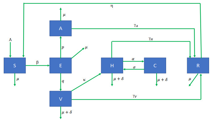
The aim of this work is to provide a new mathematical model that studies transmission dynamics of Coronavirus disease 2019 (COVID-19) caused by severe acute respiratory syndrome coronavirus 2 (SARS-CoV-2). The model captures the dynamics of the disease taking into consideration some measures and is represented by a system of nonlinear ordinary differential equations including seven classes, which are susceptible class (S), exposed class (E), asymptomatic infected class (A), severely infected class (V), hospitalized class (H), hospitalized class but in ICU (C) and recovered class (R). We prove positivity and boundedness of solutions, compute the basic reproduction number, and investigate asymptotic stability properties of the proposed model. As a consequence, dynamical properties of the model are established fully and some mitigation and prevention measures of COVID-19 outbreaks are also suggested. Furthermore, the model is fitted to COVID-19 confirmed cases in South Africa during the Omicron wave from November 27, 2021 to January 20, 2022 which helped determine the model parameters value for our numerical simulation. A set of numerical experiments using real data is conducted to support and illustrate the theoretical findings. Numerical simulation results show that fast waning of infection-induced immunity can increase the occurrence of outbreaks.

Keywords:

Citation: Oluwaseun F. Egbelowo, Justin B. Munyakazi, Manh Tuan Hoang. Mathematical study of transmission dynamics of SARS-CoV-2 with waning immunity[J]. AIMS Mathematics, 2022, 7(9): 15917-15938. doi: 10.3934/math.2022871

Related Papers:

[1]	C. W. Chukwu, Fatmawati . Modelling fractional-order dynamics of COVID-19 with environmental transmission and vaccination: A case study of Indonesia. AIMS Mathematics, 2022, 7(3): 4416-4438. doi: 10.3934/math.2022246
[2]	Ahmed M. Elaiw, Amani S. Alsulami, Aatef D. Hobiny . Global properties of delayed models for SARS-CoV-2 infection mediated by ACE2 receptor with humoral immunity. AIMS Mathematics, 2024, 9(1): 1046-1087. doi: 10.3934/math.2024052
[3]	Tahir Khan, Fathalla A. Rihan, Muhammad Bilal Riaz, Mohamed Altanji, Abdullah A. Zaagan, Hijaz Ahmad . Stochastic epidemic model for the dynamics of novel coronavirus transmission. AIMS Mathematics, 2024, 9(5): 12433-12457. doi: 10.3934/math.2024608
[4]	A. M. Elaiw, A. S. Shflot, A. D. Hobiny . Stability analysis of SARS-CoV-2/HTLV-I coinfection dynamics model. AIMS Mathematics, 2023, 8(3): 6136-6166. doi: 10.3934/math.2023310
[5]	Maryam Amin, Muhammad Farman, Ali Akgül, Mohammad Partohaghighi, Fahd Jarad . Computational analysis of COVID-19 model outbreak with singular and nonlocal operator. AIMS Mathematics, 2022, 7(9): 16741-16759. doi: 10.3934/math.2022919
[6]	S. M. E. K. Chowdhury, J. T. Chowdhury, Shams Forruque Ahmed, Praveen Agarwal, Irfan Anjum Badruddin, Sarfaraz Kamangar . Mathematical modelling of COVID-19 disease dynamics: Interaction between immune system and SARS-CoV-2 within host. AIMS Mathematics, 2022, 7(2): 2618-2633. doi: 10.3934/math.2022147
[7]	Afnan Al Agha, Hakim Al Garalleh . Oncolysis by SARS-CoV-2: modeling and analysis. AIMS Mathematics, 2024, 9(3): 7212-7252. doi: 10.3934/math.2024351
[8]	Sara J Hamis, Fiona R Macfarlane . A single-cell mathematical model of SARS-CoV-2 induced pyroptosis and the effects of anti-inflammatory intervention. AIMS Mathematics, 2021, 6(6): 6050-6086. doi: 10.3934/math.2021356
[9]	Kai Zhang, Xinzhu Meng, Abdullah Khames Alzahrani . The ACE2 receptor protein-mediated SARS-CoV-2 infection: dynamic properties of a novel delayed stochastic system. AIMS Mathematics, 2024, 9(4): 8104-8133. doi: 10.3934/math.2024394
[10]	Muhammad Altaf Khan, Sajjad Ullah, Saif Ullah, Muhammad Farhan . Fractional order SEIR model with generalized incidence rate. AIMS Mathematics, 2020, 5(4): 2843-2857. doi: 10.3934/math.2020182

Abstract

1. Introduction

Mathematical modeling and analysis can provide us with characteristic properties of important phenomena and processes arising in real-world situations as well as predict the possible scenarios in reality (see, for example, ^{[1,2,3,4,5,6,7,8,9,10,11,12]}. In particular, the study of mathematical models describing infectious diseases has become one of the powerful and effective approaches to analyze, understand and predict transmission mechanisms as well as characteristics of infectious diseases. For many years, a great number of mathematical models of infectious diseases have been constructed and studied by many mathematicians, biologists, and epidemiologists (see, for example, ^{[1,2,3,4,8,9,10]} and references therein). Studying these models can provide us with suitable strategies for controlling and preventing diseases and for protecting the public health. In recent works ^[13,14,15] we have studied some epidemic models and their real-world applications.

In March 11, 2020, the World Health Organization (WHO) declared the Coronavirus disease 2019 (COVID-19) caused by severe acute respiratory syndrome coronavirus 2 (SARS-CoV-2) outbreak a global pandemic ^[16] and in terms of the number of people infected, deaths, and the unprecedented demand for healthcare services, COVID-19 had appeared in the top 10 worst infectious disease pandemic in history in just less than 2 years after the first case was detected. Similarly to the previous outbreak of other diseases, mathematical modeling and analysis of SARS-CoV-2 epidemic has strongly attracted the attention of many researchers with many useful applications in both theory and practice, especially in disease prevention. Consequently, a large number of mathematical models of COVID-19 corresponding to different strategies have been proposed analyzed by many infectious disease experts (see, for instance, ^{[17,18,19,20,21,22,23,24,25,26,27,28,29,30,31,32,33,34,35]} and references therein).

It is worth noting that the mathematical models of the COVID-19 transmission are constructed based on principles of mathematics of epidemics, strategies and measures for combating the epidemic. Therefore, strategies for confronting the COVID-19 epidemic of each country/region may lead to a different mathematical model. In other words, there can be many mathematical models of COVID-19 transmission depending on strategies and measures for confronting the COVID-19 epidemic. Motivated and inspired by the importance of mathematical models of epidemics, we provide in this work a new mathematical study for the transmission dynamics of SARS-CoV-2. More clearly, a new mathematical model describing transmission dynamics of SARS-CoV-2 epidemic is formulated and analyzed rigorously. This model is based on hypothesis that COVID-19 has threatened to collapse hospital and ICU services in most of nations of the world and it has affected the care programs for non-COVID-19 patients ^[36]. Hence, mathematical model designed to optimize predictions related to the need for hospitalization and ICU admission by COVID-19 patients will of great important. Mathematical model of COVID-19 dynamics represented by a system of nonlinear ordinary differential equations including seven classes, which are susceptible class (S), exposed class (E), asymptomatic infected class (A), severely infected class (V), hospitalized class (H), hospitalized class but in ICU (C) and recovered class (R). The positivity and boundedness of the new proposed model are established based on comparison principles for ODEs, and its basic reproduction number is calculated by using the approach developed in ^[37]. Next, the asymptotic stability properties of the model are investigated by the Lyapunov stability theory and the relationship between the basic reproduction number and global stability of disease free equilibrium. As an important consequence, dynamical properties of the model are established fully and some mitigation and prevention measures of COVID-19 outbreaks are also suggested. In addition, a set of numerical simulations using real data is reported to support and illustrate the theoretical results. The obtained results indicate that there is a good agreement between numerical simulation results and the theoretical ones. The plan of this work is as follows. The mathematical model is formulated in Section 2. Dynamics of the proposed models is analyzed in Section 3. Numerical experiments are reported in Section 4. The last section provides some remarks and conclusion.

2. Model formulation

In this section, we formulate mathematical model for transmission dynamics of COVID-19. In this model, the total population is divided into seven classes. The mathematical model transitions through the following classes: Susceptible (S), Exposed (E), asymptomatic (A), severely infected (V), hospitalized in general ward (H), hospitalized in ICU (C) and recovered (R). The model assume that recovered individuals experiences immunity waning, $\eta$ ^[38]. The model has a constant recruitment rate $\Lambda$ to the susceptible class, S. The transmission rate from asymptomatic, A, and severely infected individuals, V, to susceptible individuals, S is given by $\beta$ with a modification parameters $\epsilon$ $(0 < \epsilon < 1)$ on $\beta$ for the severely infected individuals since it generally assumed that the asymptomatic individuals are more infectious than the symptomatic individuals ^[20]. The asymptomatic, severely infected and hospitalized individuals transit to the recovered class at rate $\gamma_A$ , $\gamma_V$ and $\gamma_H$ , respectively. It is assumed that those individuals severely infected, hospitalized in general ward and hospitalized in ICU can die due to COVID-19 disease at rate $\delta$ ^[39]. $p$ and $q$ is the rate at which exposed individual transit to asymptomatic and severely infected individuals, respectively. We considered demographic factor such as natural death in each of the class as rate $\mu.$ Severely infected individuals are hospitalized at rate $\kappa$ and hospitalized individuals transit to ICU at rate, $\alpha$ while the those recovered from ICU return to the hospital general wards at rate, $\sigma$ . In the model, we do not consider non-pharmaceutical intervention such as isolation or lockdowns.

Following Figure 1 and Table 1, the dynamics of COVID-19 transmission is modeled by the following system of nonlinear ordinary differential equations:

$\begin{equation} \begin{split} \frac{dS}{dt}& = \Lambda-\mu S -\beta A S-\beta E S-\beta \epsilon V S+ \eta R, \\ \frac{dE}{dt}& = \beta A S+\beta E S+\beta \epsilon VS-p E-q E -\mu E, \\ \frac{dA}{dt}& = p E-\gamma_A A -\mu A, \\ \frac{dV}{dt}& = q E-\kappa V-\gamma_V V-(\mu+\delta) V, \\ \frac{dH}{dt}& = \kappa V+\sigma C-\alpha H -\gamma_H H -(\mu+\delta)H, \\ \frac{dC}{dt}& = \alpha H -\sigma C-(\mu+\delta)C, \\ \frac{dR}{dt}& = \gamma_A A +\gamma_V V+\gamma_H H -\mu R- \eta R, \end{split} \end{equation}$

(2.1)

Figure 1. Compartment representation of COVID-19 transmission dynamics.

DownLoad: Full-Size Img PowerPoint

Table 1. Parameter symbols and their descriptions.

Symbol	Description
$S$	Susceptible class
$E$	Exposed class
$A$	Asymptomatic infected class
$V$	Severely infected class
$H$	Hospitalized class
$C$	Hospitalized class but in ICU
$R$	Recovered class
$\beta$	Rate at which infected individuals infect susceptibles
$p$	Proportion of asymptomatic infected
$q$	Proportion of severe infected
$\kappa$	Proportion of severe progressing to hospitalise
$\alpha$	Proportion of hospitalise progressing to critical
$\sigma$	Proportion of critical progressing to hospitalise
$\gamma_A$	Recovery proportion of asymptomatic
$\gamma_V$	Recovery proportion of mild
$\gamma_H$	Recovery proportion of severe
$\eta$	Rate of COVID-19 waning immunity
$\epsilon$	Infectious rate by the symptomatic individuals
$\mu$	Natural death rate
$\delta$	COVID-19 related death rate
$\Lambda$	Recruitment rate

| Show Table

DownLoad: CSV

subject to the initial data

$\begin{equation*} S(0) > 0, \quad E(0) \geq 0, \quad A(0) \geq 0, \quad V(0) \geq 0, \quad H(0) \geq 0, \quad C(0) \geq 0, \quad R(0) \geq 0. \end{equation*}$

The parameter $0 < \epsilon < 1$ is a modification parameter since generally the asymptomatic individuals are assumed to be more infectious than the symptomatic individuals ^[20] and $\eta$ is the rate at which those who recover from the disease become susceptible again over time ^[29].

For the model (2.1), we denote the total population by $N$ , i.e,

$\begin{equation*} N(t) : = S(t) + E(t) + A(t) + V(t) + H(t) + C(t) + R(t), \quad t \geq 0. \end{equation*}$

By using comparison theorems for ODEs ^[40], it is easy to establish the positivity and boundedness of the model as follows.

Theorem 1 (Positivity and boundedness of solutions). The set

$\begin{equation*} \mathbb{R}_+^7 : = \Big\{\big(S, E, A, V, H, I, R\big) \in \mathbb{R}^7\big|S, E, A, V, H, I, R \geq 0\Big\} \end{equation*}$

is a positively invariant set of the model (2.1). Furthermore, we have the following estimate

$\begin{equation*} \limsup\limits_{t \to \infty}N(t) \leq \dfrac{\Lambda}{\mu}. \end{equation*}$

Proof. First, it follows from (2.1) that

$\begin{equation*} \begin{split} \dfrac{dS}{dt}\Big|_{S = 0} & = \Lambda + \eta R > 0, \\ \dfrac{dE}{dt}\Big|_{E = 0} & = \beta AS + \beta\epsilon VS \geq 0, \\ \dfrac{dA}{dt}\Big|_{A = 0} & = p E \geq 0, \\ \dfrac{dV}{dt}\Big|_{V = 0} & = q E \geq 0, \\ \dfrac{dH}{dt}\Big|_{H = 0} & = \kappa V + \sigma C \geq 0, \\ \dfrac{dC}{dt}\Big|_{C = 0} & = \alpha H \geq 0, \\ \dfrac{dR}{dt}\Big|_{R = 0} & = \gamma_A A + \gamma_V V + \gamma_H H \geq 0. \end{split} \end{equation*}$

By [,Theorem B.7], we deduce that the set $\mathbb{R}^7_+$ is a positively invariant set of the model (2.1).

Next, from (2.1) we obtain

$\begin{equation*} \dfrac{dN}{dt} = \Lambda - \mu N - \delta V - \delta H - \delta C \leq \Lambda - \mu N. \end{equation*}$

By using a comparison theorem for ODEs [40,Theorem B.1], we obtain

$\begin{equation*} \limsup\limits_{t \to \infty}N(t) \leq \dfrac{\Lambda}{\mu}. \end{equation*}$

The proof is complete.

3. Dynamical analysis of the mathematical model

In this section, we will analyze dynamical properties of the model (2.1). As a consequence of Theorem 1, we only need to study dynamics of the model (2.1) on a feasible set defined by

$\begin{equation} \Omega = \bigg\{(S, E, A, V, H, C, R) \in \mathbb{R}^7_+\Big|S + E + A + V + H + C + R \leq \dfrac{\Lambda}{\mu}\bigg\}. \end{equation}$

(3.1)

3.1. Equilibria and the basic reproduction number

We solve the following non-linear algebraic system in order to determine equilibria of the model (2.1):

$\begin{equation} \begin{split} &\Lambda-\mu S -\beta A S-\beta E S-\beta \epsilon V S + \eta R = 0, \\ &\beta A S + \beta E S + \beta\epsilon VS - pE - qE - \mu E = 0, \\ &p E-\gamma_A A -\mu A = 0, \\ &q E-\kappa V-\gamma_V V-(\mu+\delta) V = 0, \\ &\kappa V+\sigma C-\alpha H -\gamma_H H -(\mu+\delta)H = 0, \\ &\alpha H -\sigma C-(\mu+\delta)C = 0, \\ &\gamma_A A +\gamma_V V + \gamma_H H -\mu R - \eta R = 0. \end{split} \end{equation}$

(3.2)

For convenience, we introduce the following notations:

$\begin{equation} \begin{split} &\tau_1 : = \dfrac{\sigma + \mu + \delta}{\alpha}, \\ &\tau_2 : = \dfrac{(\alpha + \gamma_H + \mu + \delta)\tau_1 - \sigma}{\kappa}, \\ &\tau_3 : = \dfrac{\kappa + \gamma_V + \mu + \delta}{q}\tau_2, \\ &\tau_4 : = \dfrac{p}{\gamma_A + \mu}\tau_3, \\ &\tau_5 : = \dfrac{\gamma_A\tau_4 + \gamma_V\tau_2 + \gamma_H\tau_1}{\mu + \eta}, \\ &\tau_6 : = (p + q + \mu)\tau_3 - \eta\tau_5. \end{split} \end{equation}$

(3.3)

It follows from the 6th, 5th, 4th, 3rd and 7th equations of the system (3.2) that

$\begin{equation} H = \tau_1 C, \quad V = \tau_2 C, \quad E = \tau_3 C, \quad A = \tau_4 C, \quad R = \tau_5 C. \end{equation}$

(3.4)

On the other hand, adding side-by-side the 1st and 2nd equations of (3.2) we obtain

$\begin{equation} \Lambda - \mu S = \tau_6 C. \end{equation}$

(3.5)

Combining (3.4), (3.5) with the 1st equation of (3.2) we have an equation for $C$

$\begin{equation} C\bigg[\tau_6 - \beta\bigg(\dfrac{\Lambda - \tau_6 C}{\mu}\bigg)(\epsilon\tau_2 + \tau_3 + \tau_4) +\eta\tau_5\bigg] = 0. \end{equation}$

(3.6)

The Eq (3.6) always possesses a trivial solution $C = 0$ . In this case, we have

$\begin{equation*} E_0 = A_0 = V_0 = H_0 = C_0 = R_0 = 0, \quad S_0 = \dfrac{\Lambda}{\mu}, \end{equation*}$

which corresponds to a unique disease-free equilibrium point.

Lemma 1. The model (2.1) always possesses a disease-free equilibrium (DFE) point given by

$\begin{equation} \mathcal{E}_0 = \big(S_0, \, \, E_0, \, \, A_0, \, \, V_0, \, \, H_0, \, \, C_0, \, \, R_0\big) = \bigg(\dfrac{\Lambda}{\mu}, \, \, 0, \, \, 0, \, \, 0, \, \, 0, \, \, 0, \, \, 0\bigg). \end{equation}$

(3.7)

We now use the approach developed by van den Driessche and Watmough ^[37] to compute the basic reproduction of the model. For this purpose, we set $X = (E, A, V, H, C, R, S)$ and rewrite the model (2.1) in the matrix form

$\begin{equation*} \label{eq:9} \dfrac{dX}{dt} = \mathcal{F}(X) - \mathcal{V}(X), \end{equation*}$

where

$\begin{equation*} X = \begin{pmatrix} E\\ &\\ A\\ &\\ V\\ &\\ H\\ &\\ C\\ &\\ R\\ &\\ S \end{pmatrix}, \quad \mathcal{F} = \begin{pmatrix} \beta ES + \beta SA + \beta\epsilon SV\\ &\\ 0\\ &\\ 0\\ &\\ 0\\ &\\ 0\\ &\\ 0\\ &\\ 0 \end{pmatrix},\\ \quad \mathcal{V} = \begin{pmatrix} (p + q + \mu) E\\ &\\ -p E + (\gamma_A + \mu) A\\ &\\ -q E + (\kappa + \gamma_V + \mu + \delta) V\\ &\\ -\kappa V -\sigma C+ (\mu + \delta + \alpha + \gamma_H)H\\ &\\ -\alpha H + (\sigma+\mu + \delta )C\\ &\\ -\gamma_A A - \gamma_V V - \gamma_V H + \mu R + \eta R\\ &\\ -\Lambda + \mu S +\beta SE+ \beta SA + \beta\epsilon SV - \eta R \end{pmatrix}. \end{equation*}$

At the equilibrium point $\mathcal{E}_0$ , we obtain

$\begin{equation*} \label{eq:11} F = \begin{pmatrix} \dfrac{\beta \Lambda}{\mu}&\dfrac{\beta \Lambda}{\mu} &\dfrac{\beta\epsilon \Lambda}{\mu}\\ &&\\ 0&0&0\\ &&\\ 0&0&0 \end{pmatrix}, \quad V = \begin{pmatrix} p + q + \mu&0&0\\ &&\\ -p&\mu + \gamma_A&0\\ &&\\ -q&0&\kappa + \mu + \delta + \gamma_V \end{pmatrix}. \end{equation*}$

Consequently, the basic reproduction number of the model can be computed by

$\begin{equation} \mathcal{R}_0 = \rho(FV^{-1}) = \dfrac{\beta \Lambda }{\mu(p+q+\mu)}+\dfrac{\beta \Lambda p}{\mu(p+q+\mu)(\gamma_A+\mu)} + \dfrac{\beta \Lambda q\epsilon}{\mu(p+q+\mu)(\kappa+\gamma_V+\mu+\delta)}, \end{equation}$

(3.8)

which is the number of secondary SARS-CoV-2 infections caused by one infectious individual during the infectious period in a completely susceptible population ^[32].

We now determine disease-endemic equilibrium (DEE) points by reconsidering (3.6). By simple algebraic manipulation, we obtain the non-trivial solution

$\begin{equation} C_* = \dfrac{\Lambda}{\tau_6} - \dfrac{(\tau_6 + \eta\tau_5)\mu}{\beta\tau_6(\epsilon\tau_2 + \tau_3 + \tau_4)}. \end{equation}$

(3.9)

It is easy to verify that $C_* > 0$ if and only if $\mathcal{R}_0 > 1$ . In this case, we obtain a unique (positive) DEE point by using (3.4) and (3.5).

Lemma 2. If $\mathcal{R}_0 > 1$ , then the model (2.1) has a unique DEE point $\mathcal{E}_* = (S_*, \, \, E_*, \, \, A_*, \, \, V_*, \, \, H_*, \, \, C_*, \, \, R_*)$ , where $C_*$ is given by (3.9), $E_*, A_*, V_*, H_*, R_*$ are given by (3.4) and $S_*$ is given by (3.5).

Combining Lemmas 1 and 2, we have the following result.

Theorem 2. The model (2.1) always possess a DFE point $\mathcal{E}_0$ for all values of the parameters, whereas, the unique DEE point $\mathcal{E}_*$ exists if and only if $\mathcal{R}_0 > 1$ .

3.2. Stability analysis

In this subsection, we analyze asymptotic stability of the model (2.1). For convenience, let us denote

$\begin{equation*} \begin{split} &\zeta_1 : = p + q + \mu, \\ &\zeta_2 : = \gamma_A + \mu, \\ &\zeta_3 : = \kappa + \gamma_V + \mu + \delta, \\ &\zeta_4 : = \gamma_V +\delta+\kappa. \end{split} \end{equation*}$

Theorem 3 (Local stability of the DFE point). The DFE point of the model (2.1) is locally asymptotically stable if $\mathcal{R}_0 < 1$ and unstable if $\mathcal{R}_0 > 1$ .

Proof. The Jacobian matrix of the model (2.1) evaluating at the DFE point is given by

$\begin{equation*} \label{eq:11a} J(\mathcal{E}_0) = \begin{pmatrix} -\mu&-\dfrac{\beta \Lambda}{\mu}&-\dfrac{\beta \Lambda}{\mu}&-\dfrac{\beta\epsilon \Lambda}{\mu}&0&0&\eta\\ &&&&&&\\ 0&\dfrac{\beta \Lambda}{\mu} -\zeta_1&\dfrac{\beta \Lambda}{\mu}&\dfrac{\beta\epsilon \Lambda}{\mu}&0&0&0\\ &&&&&&\\ 0&p&-\zeta_2&0&0&0&0\\ &&&&&&\\ 0&q&0&-\zeta_3&0&0&0&\\ &&&&&&\\ 0&0&0&\kappa&-(\alpha+\gamma_H +\mu+ \delta)&\sigma&0\\ &&&&&&\\ 0&0&0&0&\alpha&-(\sigma+\mu + \delta )&0\\ &&&&&&\\ 0&0&\gamma_A&\gamma_V&\gamma_H&0&-(\mu + \eta) \end{pmatrix}. \end{equation*}$

We now determine eigenvalues of $J(\mathcal{E}_0)$ . Since $J(\mathcal{E}_0)$ is a block matrix, it is sufficient to determine eigenvalues of the three following sub-matrices

$\begin{equation*} J_0 = \begin{pmatrix} -\mu \end{pmatrix}, \end{equation*}$

and

$\begin{equation} J_1 = \begin{pmatrix} \dfrac{\beta \Lambda}{\mu}-\zeta_1&\dfrac{\beta \Lambda}{\mu} &\dfrac{\beta \epsilon\Lambda}{\mu} \\ &&&\\ p&-\zeta_2&0\\ &&&\\ q&0&-\zeta_3 \end{pmatrix}, \end{equation}$

(3.10)

and

$\begin{equation} J_2 = \begin{pmatrix} -(\alpha + \gamma_H + \mu + \delta)&\sigma&0\\ &&\\ \alpha&-(\sigma +\mu+ \delta)&0\\ &&\\ \gamma_H&0&-(\mu + \eta) \end{pmatrix}. \end{equation}$

(3.11)

The matrix $J_0$ has only one eigenvalue $-\mu < 0$ . Meanwhile, the matrix $J_2$ has an eigenvalue is $-(\mu + \eta) < 0$ , and the remaining eigenvalues are the ones of the sub-matrix

$\begin{equation} J_2' = \begin{pmatrix} -(\alpha + \gamma_H + \mu + \delta)&\sigma\\ &&\\ \alpha&-(\sigma+\mu + \delta)\\ \end{pmatrix}. \end{equation}$

(3.12)

Since $\det(J_2') > 0$ and $tr(J_2') < 0$ , real parts of two eigenvalues of $J_2'$ are all negative. Consequently, real parts of three eigenvalues of $J_2$ are all negative.

On the other hand, thanks to Schur-Cohn criterion (see ^[1]) it is easy to verify that if $\mathcal{R}_0 < 1$ then real parts of all the eigenvalues of $J_1$ are negative. Hence, the local asymptotic stability of $\mathcal{E}_0$ is proved.

We now study the global stability of the DEE point based on the approach constructed by Castillo-Chavez et al. ^[41]. For this reason, consider a system of ODEs of the form

$\begin{equation} \begin{split} \dfrac{dx}{dt} & = F(x, \textbf{I}), \\ \dfrac{d\textbf{I}}{dt} & = G(x, \textbf{I}), \quad G(x, 0) = 0, \end{split} \end{equation}$

(3.13)

where $x \in \mathbb{R}^m$ denotes (its components) the number of uninfected individuals and $\textbf{I} \in \mathbb{R}^n$ denotes (its components) the number of infected individuals including latent, infectious, etc. Let $U_0 = (x^*, 0)$ be the disease-free equilibrium and $\mathcal{R}_0$ be the basic reproduction number of this system.

The conditions (H1) and (H2) below must be met to guarantee local asymptotic stability.

(H1) For $\dfrac{dx}{dt} = F(x, 0)$ , $x^*$ is globally asymptotically stable (g.a.s.).

(H2) $G(x, \textbf{I}) = A\textbf{I} - \widehat{G}(x, \textbf{I})$ , $\widehat{G}(x, \textbf{I}) \geq 0$ for $(x, \textbf{I}) \in \Omega$ ,

where $A = D_\textbf{I}G(x^*, 0)$ is an M-matrix (the off diagonal elements of A are nonnegative) and $\Omega$ is the region where the model makes biological sense.

Corollary 1 (^[41]). The fixed point $U_0 = (x^*, 0)$ is a globally asymptotic stable (g.a.s.) equilibrium of (3.13) provided that $\mathcal{R}_0 < 1$ (l.a.s.) and that assumptions (H1) and (H2) are satisfied.

Theorem 4 (Global asymptotic stability of the DFE point). The DFE point $\mathcal{E}_0$ of the model (2.1) is globally asymptotically stable if $\mathcal{R}_0 < 1$ .

Proof. First, we rewrite the model (2.1) in the form (3.13) by setting $x = S$ and $\textbf{I} = (E, A, V, H, C, R)$ . Then, the DFE point becomes $U_0 = (x^*, 0) = (\Lambda/\mu, 0)$ and the system ${dx}/{dt} = F(x, 0)$ becomes

$\begin{equation*} \dfrac{dS}{dt} = \Lambda - \mu S. \end{equation*}$

This equation has a unique equilibrium point $x^* = \Lambda/\mu$ , which is globally asymptotically stable. Therefore, the condition $(H1)$ is satisfied.

We now verify the condition $(H2)$ . For the model (2.1), we have

$\begin{equation*} \label{eq:24} G(x, \textbf{I}) = \begin{pmatrix} \beta A S+\beta E S+\beta\epsilon VS-p E-q E -\mu E\\ \\ p E-\gamma_A A -\mu A\\ \\ q E-\kappa V-\gamma_V V-(\mu+\delta) V\\ \\ \kappa V+\sigma C-\alpha H -\gamma_H H -(\mu+\delta)H\\ \\ \alpha H -\sigma C-(\mu+\delta)C\\ \\ \gamma_A A +\gamma_V V+\gamma_H H -\mu R - \eta R \end{pmatrix}, \end{equation*}$

and

$\begin{equation*} \label{eq:25} D_\textbf{I}G(x^*, 0) = \begin{pmatrix} \beta\dfrac{\Lambda}{\mu} - \zeta_1&\beta\dfrac{\Lambda}{\mu}&\beta\epsilon\dfrac{\Lambda}{\mu}&0&0&0\\ &&&&&\\ p&-\zeta_2&0&0&0&0\\ &&&&&\\ q&0&-\zeta_3&0&0&0\\ &&&&&\\ 0&0&\kappa&-\alpha - \gamma_H - (\mu + \delta)&\sigma&0\\ &&&&&\\ 0&0&0&\alpha&-(\sigma + \mu + \delta)&0\\ &&&&&\\ 0&\gamma_A&\gamma_V&\gamma_H&0&-(\mu + \eta) \end{pmatrix}. \end{equation*}$

Clearly, all the off diagonal elements of $A : = G(x, \textbf{I})$ are non-negative. Furthermore, we have

$\begin{equation} \widehat{G} = A\textbf{I} - G(x, \textbf{I}) = \begin{pmatrix} \beta E\bigg(\dfrac{\Lambda}{\mu} - S\bigg) + \beta A\bigg(\dfrac{\Lambda}{\mu} - S\bigg) + \beta\epsilon V \bigg(\dfrac{\Lambda}{\mu} - S\bigg)\\ \\ 0\\ \\ 0\\ \\ 0\\ \\ 0\\ \\ 0 \end{pmatrix}, \end{equation}$

(3.14)

which implies that $\widehat{G}(x, \textbf{I}) \geq 0$ for all $(x, \textbf{I}) \in \Omega$ . Therefore, the conditions (H1) and (H2) are satisfied. By Corollary 1 the global stability of the DEE point is obtained. The proof is complete.

Remark 1. In order to investigate the local stability of $J(\mathcal{E}_*)$ , we consider the Jacobian of the model (2.1) at $\mathcal{E}_*$ , which is given by

Note that the DEE point exists if and only if $\mathcal{R}_0 > 1$ . Since $J(\mathcal{E}_*)$ is very complicated, it is very difficult to have a format proof which shows that all the eigenvalues of $J(\mathcal{E}_*)$ have negative real parts. However, based on existing results on the asymptotic stability of mathematical models arising in biology, ecology and epidemiology (see, for instance, ^{[1,2,3,4,8,9,10]}), we can conjecture that the DEE point is not only locally asymptotically stable but also globally asymptotically stable if $\mathcal{R}_0 > 1$ . Furthermore, in numerical examples performed in the next section, we will see that $\mathcal{E}_*$ is asymptotically stable when $\mathcal{R}_0 > 1$ . The asymptotic stability analysis of the DEE point is an interesting mathematical problem but in real-world applications, our main objective is to control the parameters by suitable strategies such that $\mathcal{R}_0 \leq 1$ . In this case, the DFE point is globally stable, i.e, the disease is eradicated.

3.3. Sensitivity of the basic reproduction number

Sensitivity analysis studies how uncertainty in the output of a model can be apportioned to different source of uncertainty in the model input. It is commonly used to determine the robustness of model predictions to parameter values. In this study, the normalized forward sensitivity index of $\mathcal{R}_0$ will be computed to identify parameters that have a high influence on $\mathcal{R}_0$ . This can be used to improve intervention strategies. The normalized forward sensitivity index of a variable to a parameter is the ratio of the relative change in the variable to the relative change in the parameter ^[19].

Definition 1. (see ^[19]) The normalized forward sensitivity index of a variable, $L$ , that depends differentiably on a parameter, $u$ , is defined as:

$\begin{equation*} \label{eq:27} \Upsilon_u^{L} = \dfrac{u}{L} \dfrac{\partial L}{\partial u}. \end{equation*}$

The formula (1) evaluates the sensitivity of an outcome to all input variables. Given the basic reproduction number $\mathcal{R}_0$ above, we derive the sensitivity index of $\mathcal{R}_0$ with respect to each parameters in $\mathcal{R}_0$ as follows.

$\Upsilon_\beta^{\mathcal{R}_0} = \dfrac{\beta}{\mathcal{R}_0} \dfrac{\partial \mathcal{R}_0}{\partial \beta} = 1, \\ \Upsilon_\Lambda^{\mathcal{R}_0} = \dfrac{\Lambda}{\mathcal{R}_0} \dfrac{\partial \mathcal{R}_0}{\partial \Lambda} = 1, \\ \Upsilon_p^{\mathcal{R}_0} = \dfrac{p}{\mathcal{R}_0} \dfrac{\partial \mathcal{R}_0}{\partial p} = -{\frac { \left( \left( \left( \epsilon-1 \right) q+{\it \gamma_A} \right) \mu+ \left( q\epsilon+\delta+{\it \gamma_V}+\kappa \right) {\it \gamma_A} \mbox{}-q \left( {\it \gamma_V}+\delta+\kappa \right) \right) p}{ \left( {\mu}^{2}+ \left( q\epsilon+\delta+{\it \gamma_A}+{\it \gamma_V}+\kappa+p \right) \mu+ \left( q\epsilon+\delta+{\it \gamma_V}+\kappa \right) {\it \gamma_A}+p \zeta_4 \right) \zeta_1 }}, \\ \Upsilon_q^{\mathcal{R}_0} = \dfrac{q}{\mathcal{R}_0} \dfrac{\partial \mathcal{R}_0}{\partial q} = {\frac {q \left( \left( \epsilon-1 \right) {\mu}^{2}+ \left( \left( \epsilon-1 \right) {\it \gamma_A}+ \left( \epsilon-1 \right) p-{\it \gamma_V}-\delta-\kappa \mbox{} \right) \mu+ \left( \epsilon\, p-\delta-{\it \gamma_V}-\kappa \right) {\it \gamma_A}-p \zeta_4 \mbox{} \right) }{ \left( {\mu}^{2}+ \left( q\epsilon+\delta+{\it \gamma_A}+{\it \gamma_V}+\kappa+p \right) \mu+ \left( q\epsilon+\delta+{\it \gamma_V}+\kappa \right) {\it \gamma_A}+p \zeta_4 \right) \zeta_1 }}, \\ \Upsilon_{\gamma_A}^{\mathcal{R}_0} = \dfrac{\gamma_A}{\mathcal{R}_0} \dfrac{\partial \mathcal{R}_0}{\partial \gamma_A} = -{\frac {{\it \gamma_A}\, p \left( \kappa+{\it \gamma_V}+\mu+\delta \right) }{ \left( {\mu}^{2}+ \left( q\epsilon+\delta+{\it \gamma_A}+{\it \gamma_V}+\kappa+p \right) \mu+ \left( q\epsilon+\delta+{\it \gamma_V}+\kappa \right) {\it \gamma_A}+p \zeta_4 \right) \mbox{} \left( {\it \gamma_A}+\mu \right) }}, \\ \Upsilon_{\gamma_V}^{\mathcal{R}_0} = \dfrac{\gamma_V}{\mathcal{R}_0} \dfrac{\partial \mathcal{R}_0}{\partial \gamma_V} = -{\frac {{\it \gamma_V}\, q\epsilon\, \left( {\it \gamma_A}+\mu \right) }{ \left( {\mu}^{2}+ \left( q\epsilon+\delta+{\it \gamma_A}+{\it \gamma_V}+\kappa+p \right) \mu+ \left( q\epsilon+\delta+{\it \gamma_V}+\kappa \right) {\it \gamma_A}+p \zeta_4 \right) \mbox{} \zeta_3 }}, \\ \Upsilon_{\kappa}^{\mathcal{R}_0} = \dfrac{\kappa}{\mathcal{R}_0} \dfrac{\partial \mathcal{R}_0}{\partial \kappa} = -{\frac {\kappa\, q\epsilon\, \left( {\it \gamma_A}+\mu \right) }{ \left( {\mu}^{2}+ \left( q\epsilon+\delta+{\it \gamma_A}+{\it \gamma_V}+\kappa+p \right) \mu+ \left( q\epsilon+\delta+{\it \gamma_V}+\kappa \right) {\it \gamma_A}+p \zeta_4 \right) \zeta_3 \mbox{}}}, \\ \Upsilon_{\delta}^{\mathcal{R}_0} = \dfrac{\delta}{\mathcal{R}_0} \dfrac{\partial \mathcal{R}_0}{\partial \delta} = -{\frac {\delta\, q\epsilon\, \left( {\it \gamma_A}+\mu \right) }{ \left( {\mu}^{2}+ \left( q\epsilon+\delta+{\it \gamma_A}+{\it \gamma_V}+\kappa+p \right) \mu+ \left( q\epsilon+\delta+{\it \gamma_V}+\kappa \right) {\it \gamma_A}+p \zeta_4 \right) \zeta_3 \mbox{}}}, \\ \Upsilon_{\epsilon}^{\mathcal{R}_0} = \dfrac{\epsilon}{\mathcal{R}_0} \dfrac{\partial \mathcal{R}_0}{\partial \epsilon} = {\frac {q\epsilon\, \left( {\it \gamma_A}+\mu \right) }{{\mu}^{2}+ \left( q\epsilon+\delta+{\it \gamma_A}+{\it \gamma_V}+\kappa+p \right) \mu \mbox{}+ \left( q\epsilon+\delta+{\it \gamma_V}+\kappa \right) {\it \gamma_A}+p \zeta_4 }}.$

provides sensitivity indices of $\mathcal{R}_0$ with respect to parameters given in Set 1 of Table 3.

Table 2. Sensitivity indices of

$\mathcal{R}_0$ with respect to parameters given in Set 1 of Table 4.

Parameter	Sensitivity Index
$\beta$	1
$\Lambda$	1
$p$	-0.181
$q$	-0.096
$\gamma_A$	-0.698
$\gamma_V$	-0.010
$\kappa$	-0.013
$\epsilon$	0.023

| Show Table

DownLoad: CSV

Table 3. The parameters used in Example 1.

Parameter	Value	Source	Parameter	Value	Source
$\beta$	$0.034$	assumed	$\mu$	$\dfrac{1}{64.13\times 365}$	Estimated
$p$	$0.1760$	^[18,19]	$\delta$	$1.7826 \times 10^{-5}$	^[18,19]
$q$	$0.0240$	^[18,19]	$\Lambda=\mu\times N(0)$	$2533.8$	Estimated
$\kappa$	$0.08$	^[18,19]	$\eta$	0.008	^[29]
$\sigma$	$0.2$	^[18,19]	$\epsilon$	$0.5$	^[42]
$\alpha$	$0.15$	^[18,19]	$\gamma_H$	$0.047$	fitted
$\gamma_A$	$0.07$	fitted	$\mathcal{R}_0$	0.61	Computed
$\gamma_V$	$0.061$	fitted

| Show Table

DownLoad: CSV

Table 4. The parameters used in Example 2.

Parameter	Value	Source	Parameter	Value	Source
$\beta$	$0.34$	fitted	$\mu$	$\dfrac{1}{64.13\times 365}$	Estimated
$p$	$0.1760$	^[18,19]	$\delta$	$1.7826 \times 10^{-5}$	^[18,19]
$q$	$0.0240$	^[18,19]	$\Lambda=\mu\times N(0)$	$2533.8$	Estimated
$\kappa$	$0.08$	^[18,19]	$\eta$	0.008	^[29]
$\sigma$	$0.2$	^[18,19]	$\epsilon$	$0.5$	^[42]
$\alpha$	$0.15$	^[18,19]	$\gamma_H$	$0.047$	fitted
$\gamma_A$	$0.07$	fitted	$\mathcal{R}_0$	6.11	Computed
$\gamma_V$	$0.061$	fitted

| Show Table

DownLoad: CSV

The implication of the above investigation for intervention strategy is that decreasing $\beta$ or $\Lambda$ by $10\%$ decreases $\mathcal{R}_0$ by $10\%$ . Also, the most negative sensitive parameter is the proportion of asymptomatic infected, $\gamma_A$ , with $\Upsilon_p^{\mathcal{R}_0} = -0.698.$ If $\gamma_A$ increase by 10%, then the basic reproduction number $\mathcal{R}_0$ decreases approximately 7%. We have not included the sensitivity index related to death rates due to ethical reasons. Therefore, compliance with COVID-19 mitigation measures such as social distancing, wearing a face mask, and washing hands is needed to reduce the transmission parameter $\beta$ ; furthermore, the spread of COVID-19 infection can be reduced by quarantining infected people and/or by using COVID-19 vaccines.

4. Numerical experiments

In this section, we provide the biological parameters of the proposed COVID-19 model (2.1) using the confirmed COVID-19 cases in South Africa during the Omicron wave period from November 27, 2021 to January 20, 2022 ^[43]. Using the using Poisson maximum likelihood and the dataset, we estimate parameter values in the model.

The initial value of the total population of South Africa based on the data is $N(0) = 59310000$ and the average life span is $\dfrac{1}{64.13}$ years. The fitting result to the reported data through our model is compared in . Hence, it can be seen that the simulation model is quite in accordance with the actual data. We perform some numerical experiments with initial condition given in . For this purpose, we utilize the classical fourth order Runge-Kutta (RK4) method with step-size $h = 10^{-4}$ to simulate the model (2.1). In addition, the following set of initial data will be also used in numerical simulations.

Figure 2. South Africa COVID-19 data between the period of November 27, 2021 and January 20, 2022 fitted to COVID-19 model.

DownLoad: Full-Size Img PowerPoint

Table 5. The initial data used in numerical examples.

$S(0)$	$E(0)$	$A(0)$	$V(0)$	$H(0)$	$C(0)$	$R(0)$	$N(0)$	Ref
29675142	21968562	2861104	715275	572220	114444	3403253	59310000	^[44]

| Show Table

DownLoad: CSV

Example 1 (The dynamics of the transmission model when $\mathcal{R}_0 < 1$ ). Consider the model (2.1) with the parameters given in . This scenario is to show the dynamic of the model when $\mathcal{R}_0 < 1$ .

In this example, $\mathcal{R}_0 < 1$ and hence, the DFE point $\mathcal{E}_0 = \Big(\dfrac{\Lambda}{\mu}, \, \, 0, \, \, 0, \, \, 0, \, \, 0, \, \, 0, \, \, 0\Big)$ is globally asymptotically stable. This implies that the epidemic will be eradicated. The solutions of the model (2.1) are depicted in Figure 3. It is clear that the DFE point is globally asymptotically stable. Therefore, the validity of Theorems 3 and 4 is supported.

Figure 3. The solutions in Example 2 with Set 2 of the initial data.

DownLoad: Full-Size Img PowerPoint

Example 2 (The dynamics of the transmission model when $\mathcal{R}_0 > 1$ ). Consider the model (2.1) with the parameters given in . This scenario is to show the dynamic of the model when $\mathcal{R}_0 > 1$ .

In this case $\mathcal{R}_0 > 1$ and therefore, the DEE point $\mathcal{E}_*$ is locally asymptotically stable. The solutions of the model are depicted in Figure 4. It is clear that the DEE point is locally asymptotically stable. This is a evidence supporting the comments in Remark 1. Also, we can observe that the DEE point may be not only locally stable but also globally stable. Based on this, it is reasonable to conjecture the global asymptotic stability of the DEE point as reported in Remark 1.

Figure 4. The solutions in Example 2 with Set 2 of the initial data.

DownLoad: Full-Size Img PowerPoint

shows that variable duration of immunity has impact on the dynamics of the diseases. If there is relatively quick loss of immunity, accumulation of susceptible individual may results in a disproportionately large outbreak in a subsequent wave. in , when $\eta = 0.0111$ , which corresponded to the fasted loss of immunity in all the $\eta$ considered, we observed accumulation of more susceptible individuals and low number of recovered individuals. shows that an increase in the transmission rate will increase the $\mathcal{R}_0$ while shows that the values of $\mathcal{R}_0$ can be kept below 1 as long as the values of transmission rate do not exceed a certain threshold $(\beta \approx 0.11)$ .

Figure 5. Variation of total number of susceptible and recovered individuals with different values of waning immunity (

$\eta$ ).

DownLoad: Full-Size Img PowerPoint

Figure 6. Contour plots of the reproduction number

$(\mathcal{R}_0)$ of the model as a function of transmission rate

$\beta$ and asymptomatic (

$\gamma_A$ ) and symptomatic (

$\gamma_V$ ).

DownLoad: Full-Size Img PowerPoint

5. Conclusions and remarks

In this work, a mathematical model of the transmission dynamics of SARS-CoV-2 epidemic has been formulated and its dynamical properties have been investigated rigorously. By the rigorous mathematical analyses, we have computed the basic reproduction number $\mathcal{R}_0$ , proved the positivity and boundedness of solutions and established the asymptotic stability properties of the DFE and DEE points. It was proved that the DFE point is globally asymptotically stable if $\mathcal{R}_0 \leq 1$ , whereas, the DEE point is locally asymptotically stable if $\mathcal{R}_0 > 1$ . The normalized sensitivity index of $\mathcal{R}_0$ has been considered. We adopted the Poisson maximum likelihood to estimate and fit the model parameters using the reported active cases of COVID-19 in South Africa. The results indicate that the use of Poisson maximum likelihood yields a good fit as shown in Figure 2. Also, we have conducted a set of numerical experiments with with estimated parameters to support and illustrate the constructed theoretical results.

The constructed model and theoretical analysis not only provide us with a new observation of the transmission dynamics of COVID-19 but also suggest effective disease prevention measures. More clearly, an important consequence obtained from the theoretical analysis is that we determined the basic reproduction number $\mathcal{R}_0$ and identified the parameters that influence the $\mathcal{R}_0$ . Based on this, some mitigation and preventative measures of COVID-19 outbreaks have been suggested. These mitigation and preventative measures can be useful in real situations and consistence with the WHO's recommendations.

In the current model, we incorporate infection-induced waning immunity. However, promising development directions for model (2.1) are to consider it along with vaccine waning immunity and optimal control strategies. Especially, in the context that the vaccination is being promoted in all countries, the study of the impact of vaccines, waning immunity and optimal control strategies are very important. This can provide us with effective vaccination strategies as well as disease prevention.

The proposed model is not exhaustive and can be extended in various ways. In the near future, we intend to develop this work to construct new mathematical models for transmission dynamics of SARS-CoV-2 epidemic and study practical applications of the proposed model. Also, pharmaceutical and non-pharmaceutical interventions, and optimal control strategies will be considered for the SARS-CoV-2 epidemic model.

Acknowledgments

The first author, Oluwaseun F. Egbelowo, acknowledges support from the DSI-NRF Centre of Excellence in Mathematical and Statistical Sciences (CoE-MaSS), South Africa. Opinions expressed and conclusions arrived at are those of the authors and are not necessarily to be attributed to the CoE-MaSS. Justin Munyakazi's research was supported by the National Research Foundation of South Africa. The authors wish to thank the editor and the anonymous reviewers for their time and for providing comments and suggestions that have helped improve the quality of this paper.

Conflict of interest

The authors declare that there is no conflict of interest regarding the publication of this paper.

References

[1]	L. J. S. Allen, Introduction to mathematical biology, Pearson, 2016.
[2]	F. Brauer, C. Castillo-Chavez, Z. Feng, Mathematical models in epidemiology, 1 Ed., Springer, 2019.
[3]	F. Brauer, Mathematical epidemiology: Past, present, and future, Infect. Dis. Model., 2 (2017), 113–127. https://doi.org/10.1016/j.idm.2017.02.001 doi: 10.1016/j.idm.2017.02.001
[4]	F. Brauer, Compartmental models in epidemiology, In: Mathematical epidemiology, Springer, Berlin, Heidelberg, 2008. https://doi.org/10.1007/978-3-540-78911-6_2
[5]	N. C. Grassly, C. Fraser, Mathematical models of infectious disease transmission, Nat. Rev. Microbiol., 6 (2008), 477–487. https://doi.org/10.1038/nrmicro1845 doi: 10.1038/nrmicro1845
[6]	K. Hattaf, H. Dutta, Mathematical modelling and analysis of infectious diseases, Springer, 2020. https://doi.org/10.1007/978-3-030-49896-2
[7]	S. Tyagi, S. C. Martha, S. Abbas, A. Debbouch, Mathematical modeling and analysis for controlling the spread of infectious diseases, Chaos, Solitons Fract., 144 (2021), 110707. https://doi.org/10.1016/j.chaos.2021.110707 doi: 10.1016/j.chaos.2021.110707
[8]	M. Y. Li, An introduction to mathematical modeling of infectious diseases, 1 Ed., Springer, 2018.
[9]	M. Martcheva, An introduction to mathematical epidemiology, 1 Ed., Springer, 2015.
[10]	M. A. Nowak, R. M. May, Viral dynamics, Oxford: Oxford University Press, 2000.
[11]	Y. Xie, Z. Wang, Transmission dynamics, global stability and control strategies of a modified SIS epidemic model on complex networks with an infective medium, Math. Comput. Simul., 188 (2021), 23–34. https://doi.org/10.1016/j.matcom.2021.03.029 doi: 10.1016/j.matcom.2021.03.029
[12]	Y. Xie, Z. Wang, A ratio-dependent impulsive control of an SIQS epidemic model with non-linear incidence, Appl. Math. Comput., 423 (2022), 127018. https://doi.org/10.1016/j.amc.2022.127018 doi: 10.1016/j.amc.2022.127018
[13]	M. T. Hoang, O. F. Egbelowo, Nonstandard finite difference schemes for solving an SIS epidemic model with standard incidence, Rend. Circ. Mat. Palermo, Ser. II, 69 (2020), 753–769. https://doi.org/10.1007/s12215-019-00436-x doi: 10.1007/s12215-019-00436-x
[14]	M. T. Hoang, O. F. Egbelowo, On the global asymptotic stability of a hepatitis B epidemic model and its solutions by nonstandard numerical schemes, Bol. Soc. Mat. Mex., 26 (2020), 1113–1134. https://doi.org/10.1007/s40590-020-00275-2 doi: 10.1007/s40590-020-00275-2
[15]	M. T. Hoang, O. F. Egbelowo, Dynamics of a fractional-order hepatitis b epidemic model and its solutions by nonstandard numerical schemes, In: K. Hattaf, H. Dutta, Mathematical modelling and analysis of infectious diseases, Studies in Systems, Decision and Control, Springer, 2020. https://doi.org/10.1007/978-3-030-49896-2_5
[16]	WHO Director-General's opening remarks at the media briefing on COVID19-March 2020, 2020. Available from: https://www.who.int/director-general/speeches/detail/who-director-general-s-opening-remarks-at-the-media-briefing-on-covid-19---20-march-2020.
[17]	A. Anirudh, Mathematical modeling and the transmission dynamics in predicting the Covid-19-What next in combating the pandemic, Infect. Dis. Model., 5 (2020), 366–374. https://doi.org/10.1016/j.idm.2020.06.002 doi: 10.1016/j.idm.2020.06.002
[18]	M. Kimathi, S. Mwalili, V. Ojiambo, D. K. Gathungu, Age-structured model for COVID-19: Effectiveness of social distancing and contact reduction in Kenya, Infect. Dis. Model., 6 (2021), 15–23. https://doi.org/10.1016/j.idm.2020.10.012 doi: 10.1016/j.idm.2020.10.012
[19]	O. Iyiola, B. Oduro, T. Zabilowicz, B. Iyiola, D. Kenes, System of time fractional models for COVID-19: Modeling, analysis and solutions, Symmetry, 13 (2021), 787. https://doi.org/10.3390/sym13050787 doi: 10.3390/sym13050787
[20]	M. Kinyili, J. B. Munyakazi, A. Y. A. Mukhtar, Assessing the impact of vaccination on COVID-19 in South Africa using mathematical modeling, Appl. Math. Inf. Sci., 15 (2021), 701–716. https://doi.org/10.18576/amis/150604 doi: 10.18576/amis/150604
[21]	V. S. Panwar, P. S. Sheik Uduman, J. F. Gomez-Aguilar, Mathematical modeling of coronavirus disease COVID-19 dynamics using CF and ABC non-singular fractional derivatives, Chaos, Solitons Fract., 145 (2021), 110757. https://doi.org/10.1016/j.chaos.2021.110757 doi: 10.1016/j.chaos.2021.110757
[22]	R. K. Rai, S. Khajanchi, P. K. Tiwari, E. Venturino, A. K. Misra, Impact of social media advertisements on the transmission dynamics of COVID-19 pandemic in India, J. Appl. Math. Comput., 68 (2022), 19–44. https://doi.org/10.1007/s12190-021-01507-y doi: 10.1007/s12190-021-01507-y
[23]	A. ul Rehman, R. Singh, P. Agarwal, Modeling, analysis and prediction of new variants of COVID-19 and dengue co-infection on complex network, Chaos, Solitons Fract., 150 (2021), 111008. https://doi.org/10.1016/j.chaos.2021.111008 doi: 10.1016/j.chaos.2021.111008
[24]	M. Serhani, H. Labbardi, Mathematical modeling of COVID-19 spreading with asymptomatic infected and interacting peoples, J. Appl. Math. Comput., 66 (2021), 1–20. https://doi.org/10.1007/s12190-020-01421-9 doi: 10.1007/s12190-020-01421-9
[25]	Y. Guo, T. Li, Modeling and dynamic analysis of novel coronavirus pneumonia (COVID-19) in China, J. Appl. Math. Comput., 2021. https://doi.org/10.1007/s12190-021-01611-z
[26]	S. He, Y. Peng, K. Sun, SEIR modeling of the COVID-19 and its dynamics, Nonlinear Dyn., 101 (2020), 1667–1680. https://doi.org/10.1007/s11071-020-05743-y doi: 10.1007/s11071-020-05743-y
[27]	S. Annas, M. I. Pratama, M. Rifandi, W. Sanusi, S. Side, Stability analysis and numerical simulation of SEIR model for pandemic COVID-19 spread in Indonesia, Chaos, Solitons Fract., 139 (2020), 110072. https://doi.org/10.1016/j.chaos.2020.110072 doi: 10.1016/j.chaos.2020.110072
[28]	B. A. Baba, B. Bilgehan, Optimal control of a fractional order model for the COVID-19 pandemic, Chaos, Solitons Fract., 144 (2021), 110678. https://doi.org/10.1016/j.chaos.2021.110678 doi: 10.1016/j.chaos.2021.110678
[29]	D. Dwomoh, S. Iddi, B. Adu, J. M. Aheto, K. M. Sedzro, J. Fobil, et al., Mathematical modeling of COVID-19 infection dynamics in Ghana: Impact evaluation of integrated government and individual level interventions, Infect. Dis. Model., 6 (2021), 381–397. https://doi.org/10.1016/j.idm.2021.01.008 doi: 10.1016/j.idm.2021.01.008
[30]	M. Higazy, Novel fractional order SIDARTHE mathematical model of COVID-19 pandemic, Chaos, Solitons Fract., 138 (2020), 110007. https://doi.org/10.1016/j.chaos.2020.110007 doi: 10.1016/j.chaos.2020.110007
[31]	M. M. Hikal, M. M. A. Elsheikh, W. K. Zahra, Stability analysis of COVID-19 model with fractional-order derivative and a delay in implementing the quarantine strategy, J. Appl. Math. Comput., 68 (2021), 295–321. https://doi.org/10.1007/s12190-021-01515-y doi: 10.1007/s12190-021-01515-y
[32]	J. M. Tchuenche, N. Dube, C. P. Bhunu, R. J. Smith, C. T. Bauch, The impact of media coverage on the transmission dynamics of human influenza, BMC Public Health, 11 (2011), 1–16. https://doi.org/10.1186/1471-2458-11-S1-S5 doi: 10.1186/1471-2458-11-S1-S5
[33]	A. R. Tuite, D. N. Fisman, A. L. Greer, Mathematical modelling of COVID-19 transmission and mitigation strategies in the population of Ontario, Canada, CMAJ, 192 (2020), E497–E505. https://doi.org/10.1503/cmaj.200476 doi: 10.1503/cmaj.200476
[34]	M. Wang, Y. Hu, L. Wu, Dynamic analysis of a SIQR epidemic model considering the interaction of environmental differences, J. Appl. Math. Comput., 2021. https://doi.org/10.1007/s12190-021-01628-4.
[35]	Z. Zhang, A. Zeb, O. F. Egbelowo, V. S. Erturk, Dynamics of a fractional order mathematical model for COVID-19 epidemic, Adv. Differ. Equ., 2020 (2020), 1–16. https://doi.org/10.1186/s13662-020-02873-w doi: 10.1186/s13662-020-02873-w
[36]	J. M. Garrido, D. Martínez-Rodríguez, F. Rodríguez-Serrano, J. M. Pérez-Villares, A. Ferreiro-Marzal, M. M. Jiménez-Quintana, et al., Mathematical model optimized for prediction and health care planning for COVID-19, Med. Intensiva, 46 (2022), 248–258. https://doi.org/10.1016/j.medin.2021.02.014 doi: 10.1016/j.medin.2021.02.014
[37]	P. van den Driessche, J. Watmough, Reproduction numbers and sub-threshold endemic equilibria for compartmental models of disease transmission, Math. Biosci., 180 (2002), 29–48. https://doi.org/10.1016/S0025-5564(02)00108-6 doi: 10.1016/S0025-5564(02)00108-6
[38]	S. Xia, K. Duan, Y. Zhang, D. Zhao, H. Zhang, Z. Xie, et al., Effect of an inactivated vaccine against SARS-CoV-2 on safety and immunogenicity outcomes: Interim analysis of 2 randomized clinical trials, JAMA, 324 (2020), 951–960. https://doi.org/10.1001/jama.2020.15543 doi: 10.1001/jama.2020.15543
[39]	G. Gonzalez-Parra, A. J. Arenas, Nonlinear dynamics of the introduction of a new SARS-CoV-2 variant with different infectiousness, Mathematics, 9 (2021), 1564. https://doi.org/10.3390/math9131564 doi: 10.3390/math9131564
[40]	H. L. Smith, P. E. Waltman, The theory of the chemostat: Dynamics of microbial competition, Cambridge University Press, 2008.
[41]	C. Castillo-Chavez, Z. Feng, W. Huang, On the computation of R0 and its role in global stability, Mathematical Approaches for Emerging and Re-emerging Infection Diseases: An Introduction, 125 (2002), 31–65.
[42]	E. A. Iboi, C. N. Ngonghala, A. B. Gumel, Will an imperfect vaccine curtail the COVID-19 pandemic in the U.S., Infect. Dis. Model., 5 (2020), 510–524. https://doi.org/10.1016/j.idm.2020.07.006 doi: 10.1016/j.idm.2020.07.006
[43]	World Health Organization. Available from: https://covid19.who.int/region/afro/country/za.
[44]	South Africa Coronavirus. Available from: https://sacoronavirus.co.za.

This article has been cited by:

1.	Victoria May P. Mendoza, Renier Mendoza, Youngsuk Ko, Jongmin Lee, Eunok Jung, Managing bed capacity and timing of interventions: a COVID-19 model considering behavior and underreporting, 2022, 8, 2473-6988, 2201, 10.3934/math.2023114
2.	Itsuki Nishimura, Md. Rajib Arefin, Yuichi Tatsukawa, Shinobu Utsumi, Md. Anowar Hossain, Jun Tanimoto, Social dilemma analysis on vaccination game accounting for the effect of immunity waning, 2023, 171, 09600779, 113426, 10.1016/j.chaos.2023.113426
3.	D. Calvetti, E. Somersalo, Post-pandemic modeling of COVID-19: Waning immunity determines recurrence frequency, 2023, 365, 00255564, 109067, 10.1016/j.mbs.2023.109067

Reader Comments

Your name:*

Email:*
© 2022 the Author(s), licensee AIMS Press. This is an open access article distributed under the terms of the Creative Commons Attribution License (http://creativecommons.org/licenses/by/4.0)

通讯作者: 陈斌, bchen63@163.com

1.
沈阳化工大学材料科学与工程学院沈阳 110142

AIMS Mathematics

1.8 3.4

Metrics

Article views(1906) PDF downloads(112) Cited by(3)

Preview PDF

Download XML

Export Citation

Article outline

Show full outline

Figures and Tables

Figures(6) / Tables(5)

AIMS Mathematics

Mathematical study of transmission dynamics of SARS-CoV-2 with waning immunity

Related Papers:

Abstract

1. Introduction

2. Model formulation

3. Dynamical analysis of the mathematical model

3.1. Equilibria and the basic reproduction number

3.2. Stability analysis

3.3. Sensitivity of the basic reproduction number

4. Numerical experiments

5. Conclusions and remarks

Acknowledgments

Conflict of interest

References

This article has been cited by:

Reader Comments

通讯作者: 陈斌, bchen63@163.com

Metrics

Figures and Tables

Other Articles By Authors

Catalog

AIMS Mathematics

Mathematical study of transmission dynamics of SARS-CoV-2 with waning immunity

Related Papers:

Abstract

1. Introduction

2. Model formulation

3. Dynamical analysis of the mathematical model

3.1. Equilibria and the basic reproduction number

3.2. Stability analysis

3.3. Sensitivity of the basic reproduction number

4. Numerical experiments

5. Conclusions and remarks

Acknowledgments

Conflict of interest

References

This article has been cited by:

Reader Comments

通讯作者: 陈斌, bchen63@163.com

Metrics

Figures and Tables

Other Articles By Authors

Related pages

Tools

Export File

Citation

Format

Content

Catalog