The coronavirus disease 2019 (COVID-19) is caused by a new coronavirus known as severe acute respiratory syndrome coronavirus 2 (SARS-CoV-2). SARS-CoV-2 infects the epithelial (target) cells by binding its spike protein, S, to the angiotensin-converting enzyme 2 (ACE2) receptor on the surface of epithelial cells. During the process of SARS-CoV-2 infection, ACE2 plays an important mediating role. In this work, we develop two models which describe the within-host dynamics of SARS-CoV-2 under the effect of humoral immunity, and considering the role of the ACE2 receptor. We consider two discrete (or distributed) delays: (ⅰ) Delay in the SARS-CoV-2 infection of epithelial cells, and (ⅱ) delay in the maturation of recently released SARS-CoV-2 virions. Five populations are considered in the models: Uninfected epithelial cells, infected cells, SARS-CoV-2 particles, ACE2 receptors and antibodies. We first address the fundamental characteristics of the delayed systems, then find all possible equilibria. On the basis of two threshold parameters, namely the basic reproduction number, $ \Re_{0} $, and humoral immunity activation number, $ \Re_{1} $, we prove the existence and stability of the equilibria. We establish the global asymptotic stability for all equilibria by constructing suitable Lyapunov functions and using LaSalle's invariance principle. To illustrate the theoretical results, we perform numerical simulations. We perform sensitivity analysis and identify the most sensitive parameters. The respective influences of humoral immunity, time delays and ACE2 receptors on the SARS-CoV-2 dynamics are discussed. It is shown that strong stimulation of humoral immunity may prevent the progression of COVID-19. It is also found that increasing time delays can effectively decrease $ \Re_{0} $ and then inhibit the SARS-CoV-2 replication. Moreover, it is shown that $ \Re_{0} $ is affected by the proliferation and degradation rates of ACE2 receptors, and this may provide worthy input for the development of possible receptor-targeted vaccines and drugs. Our findings may thus be helpful for developing new drugs, as well as for comprehending the dynamics of SARS-CoV-2 infection inside the host.
Citation: Ahmed M. Elaiw, Amani S. Alsulami, Aatef D. Hobiny. Global properties of delayed models for SARS-CoV-2 infection mediated by ACE2 receptor with humoral immunity[J]. AIMS Mathematics, 2024, 9(1): 1046-1087. doi: 10.3934/math.2024052
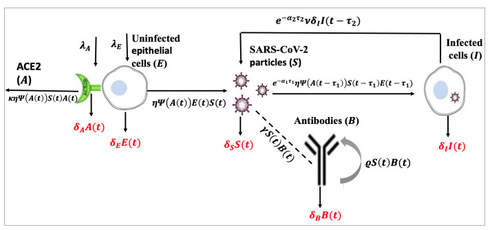
The coronavirus disease 2019 (COVID-19) is caused by a new coronavirus known as severe acute respiratory syndrome coronavirus 2 (SARS-CoV-2). SARS-CoV-2 infects the epithelial (target) cells by binding its spike protein, S, to the angiotensin-converting enzyme 2 (ACE2) receptor on the surface of epithelial cells. During the process of SARS-CoV-2 infection, ACE2 plays an important mediating role. In this work, we develop two models which describe the within-host dynamics of SARS-CoV-2 under the effect of humoral immunity, and considering the role of the ACE2 receptor. We consider two discrete (or distributed) delays: (ⅰ) Delay in the SARS-CoV-2 infection of epithelial cells, and (ⅱ) delay in the maturation of recently released SARS-CoV-2 virions. Five populations are considered in the models: Uninfected epithelial cells, infected cells, SARS-CoV-2 particles, ACE2 receptors and antibodies. We first address the fundamental characteristics of the delayed systems, then find all possible equilibria. On the basis of two threshold parameters, namely the basic reproduction number, $ \Re_{0} $, and humoral immunity activation number, $ \Re_{1} $, we prove the existence and stability of the equilibria. We establish the global asymptotic stability for all equilibria by constructing suitable Lyapunov functions and using LaSalle's invariance principle. To illustrate the theoretical results, we perform numerical simulations. We perform sensitivity analysis and identify the most sensitive parameters. The respective influences of humoral immunity, time delays and ACE2 receptors on the SARS-CoV-2 dynamics are discussed. It is shown that strong stimulation of humoral immunity may prevent the progression of COVID-19. It is also found that increasing time delays can effectively decrease $ \Re_{0} $ and then inhibit the SARS-CoV-2 replication. Moreover, it is shown that $ \Re_{0} $ is affected by the proliferation and degradation rates of ACE2 receptors, and this may provide worthy input for the development of possible receptor-targeted vaccines and drugs. Our findings may thus be helpful for developing new drugs, as well as for comprehending the dynamics of SARS-CoV-2 infection inside the host.

| [1] |
E. Vermisoglou, D. Panáček, K. Jayaramulu, M. Pykal, I. Frébort, M. Kolář, et al., Human virus detection with graphenebased materials, Biosens. Bioelectron., 166 (2020), 112436. https://doi.org/10.1016/j.bios.2020.112436 doi: 10.1016/j.bios.2020.112436

|
| [2] | World Health Organization (WHO), Coronavirus disease (COVID-19), weekly epidemiological update, 2023. Available from: https://www.who.int/publications/m/item/weekly-epidemiological-update-on-covid-19–-1-september-2023. |
| [3] |
C. B. Jackson, M. Farzan, B. Chen, H. Choe, Mechanisms of SARS-CoV-2 entry into cells, Nat. Rev. Mol. Cell Bio., 23 (2022), 3–20. https://doi.org/10.1038/s41580-021-00418-x doi: 10.1038/s41580-021-00418-x
|
| [4] |
P. Zhou, X. L. Yang, X. G. Wang, B. Hu, L. Zhang, W. Zhang, et al., A pneumonia outbreak associated with a new coronavirus of probable bat origin, Nature, 579 (2020), 270–273. https://doi.org/10.1038/s41586-020-2012-7 doi: 10.1038/s41586-020-2012-7
|
| [5] |
Y. Wan, J. Shang, R. Graham, R. S. Baric, F. Li, Receptor recognition by the novel coronavirus from Wuhan: An analysis based on decade-long structural studies of SARS coronavirus, J. Virol., 94 (2020). https://doi.org/10.1128/jvi.00127-20 doi: 10.1128/jvi.00127-20
|
| [6] |
E. A. H. Vargas, J. X. V. Hernandez, In-host mathematical modelling of COVID-19 in humans, Ann. Rev. Control, 50 (2020), 448–456. https://doi.org/10.1016/j.arcontrol.2020.09.006 doi: 10.1016/j.arcontrol.2020.09.006
|
| [7] |
C. Li, J. Xu, J. Liu, Y. Zhou, The within-host viral kinetics of SARS-CoV-2, Math. Biosci. Eng., 17 (2020), 2853–2861. https://doi.org/10.3934/mbe.2020159 doi: 10.3934/mbe.2020159
|
| [8] |
R. Ke, C. Zitzmann, D. D. Ho, R. M. Ribeiro, A. S. Perelson, In vivo kinetics of SARS-CoV-2 infection and its relationship with a person's infectiousness, P. Nat. A. Sci., 118 (2021), e2111477118. https://doi.org/10.1073/pnas.2111477118 doi: 10.1073/pnas.2111477118
|
| [9] |
M. Sadria, A. T. Layton, Modeling within-host SARS-CoV-2 infection dynamics and potential treatments, Viruses, 13 (2021), 1141. https://doi.org/10.3390/v13061141 doi: 10.3390/v13061141
|
| [10] |
I. Ghosh, Within host dynamics of SARS-CoV-2 in humans: Modeling immune responses and antiviral treatments, SN Comput. Sci., 2 (2021), 482. https://doi.org/10.1007/s42979-021-00919-8 doi: 10.1007/s42979-021-00919-8
|
| [11] |
S. Q. Du, W. Yuan, Mathematical modeling of interaction between innate and adaptive immune responses in COVID-19 and implications for viral pathogenesis, J. Med. Virol., 92 (2020), 1615–1628. https://doi.org/10.1002/jmv.25866 doi: 10.1002/jmv.25866
|
| [12] |
K. Hattaf, N. Yousfi, Dynamics of SARS-CoV-2 infection model with two modes of transmission and immune response, Math. Biosci. Eng., 17 (2020), 5326–5340. https://doi.org/10.3934/mbe.2020288 doi: 10.3934/mbe.2020288
|
| [13] |
J. Mondal, P. Samui, A. N. Chatterjee, Dynamical demeanour of SARS-CoV-2 virus undergoing immune response mechanism in COVID-19 pandemic, Eur. Phys. J.-Spec. Top., 231 (2022), 3357–3370. https://doi.org/10.1140/epjs/s11734-022-00437-5 doi: 10.1140/epjs/s11734-022-00437-5
|
| [14] |
A. E. S. Almoceraa, G. Quiroz, E. A. H. Vargas, Stability analysis in COVID-19 within-host model with immune response, Commun. Nonlinear Sci., 95 (2021), 105584. https://doi.org/10.1016/j.cnsns.2020.105584 doi: 10.1016/j.cnsns.2020.105584
|
| [15] |
A. M. Elaiw, A. J. Alsaedi, A. D. Hobiny, S. Aly, Stability of a delayed SARS-CoV-2 reactivation model with logistic growth and adaptive immune response, Physica A, 616 (2023), 128604. https://doi.org/10.1016/j.physa.2023.128604 doi: 10.1016/j.physa.2023.128604
|
| [16] |
P. Wu, X. Wang, Z. Feng, Spatial and temporal dynamics of SARS-CoV-2: Modeling, analysis and simulation, Appl. Math. Model., 113 (2023), 220–240. https://doi.org/10.1016/j.apm.2022.09.006 doi: 10.1016/j.apm.2022.09.006
|
| [17] |
A. Gonçalves, J. Bertrand, R. Ke, E. Comets, X. D. Lamballerie, D. Malvy, et al., Timing of antiviral treatment initiation is critical to reduce SARS-CoV-2 viral load, CPT-Pharmacomet. Syst., 9 (2020), 509–514. https://doi.org/10.1002/psp4.12543 doi: 10.1002/psp4.12543
|
| [18] |
P. Abuin, A. Anderson, A. Ferramosca, E. A. H. Vargas, A. H. Gonzalez, Characterization of SARS-CoV-2 dynamics in the host, Ann. Rev. Control, 50 (2020), 457–468. https://doi.org/10.1016/j.arcontrol.2020.09.008 doi: 10.1016/j.arcontrol.2020.09.008
|
| [19] |
B. Chhetri, V. M. Bhagat, D. K. K. Vamsi, V. S. Ananth, D. B. Prakash, R. Mandale, et al., Within-host mathematical modeling on crucial inflammatory mediators and drug interventions in COVID-19 identifies combination therapy to be most effective and optimal, Alex. Eng. J., 60 (2021), 2491–2512. https://doi.org/10.1016/j.aej.2020.12.011 doi: 10.1016/j.aej.2020.12.011
|
| [20] |
T. Song, Y. Wang, X. Gu, S. Qiao, Modeling the within-host dynamics of SARS-CoV-2 infection based on antiviral treatment, Mathematics, 11 (2023), 3485. https://doi.org/10.3390/math11163485 doi: 10.3390/math11163485
|
| [21] |
A. M. Elaiw, A. J. Alsaedi, A. D. Al Agha, A. D. Hobiny, Global stability of a humoral immunity COVID-19 model with logistic growth and delays, Mathematics, 10 (2022), 1857. https://doi.org/10.3390/math10111857 doi: 10.3390/math10111857
|
| [22] |
S. Tang, W. Ma, P. Bai, A novel dynamic model describing the spread of the MERS-CoV and the expression of dipeptidyl peptidase 4, Comput. Math. Method. M., 2017 (2017), 5285810. https://doi.org/10.1155/2017/5285810 doi: 10.1155/2017/5285810
|
| [23] |
T. Keyoumu, W. Ma, K. Guo, Existence of positive periodic solutions for a class of in-host MERS-CoV infection model with periodic coefficients, AIMS Math., 7 (2021), 3083–3096. https://doi.org/10.3934/math.2022171 doi: 10.3934/math.2022171
|
| [24] |
T. Keyoumu, K. Guo, W. Ma, Periodic oscillation for a class of in-host MERS-CoV infection model with CTL immune response, Math. Biosci. Eng., 19 (2022), 12247–12259. https://doi.org/10.3934/mbe.2022570 doi: 10.3934/mbe.2022570
|
| [25] |
T. Keyoumu, W. Ma, K. Guo, Global stability of a MERS-CoV infection model with CTL immune response and intracellular delay, Mathematics, 11 (2023), 1066. https://doi.org/10.3390/math11041066 doi: 10.3390/math11041066
|
| [26] |
A. N. Chatterjee, F. Al Basir, A model for SARS-CoV-2 infection with treatment, Comput. Math. Method. M., 2020 (2020), 1352982. https://doi.org/10.1155/2020/1352982 doi: 10.1155/2020/1352982
|
| [27] |
J. Lv, W. Ma, Global asymptotic stability of a delay differential equation model for SARS-CoV-2 virus infection mediated by ACE2 receptor protein, Appl. Math. Lett., 142 (2023), 108631. https://doi.org/10.1016/j.aml.2023.108631 doi: 10.1016/j.aml.2023.108631
|
| [28] |
N. Bairagi, D. Adak, Global analysis of HIV-1 dynamics with Hill type infection rate and intracellular delay, Appl. Math. Model., 38 (2014), 5047–5066. https://doi.org/10.1016/j.apm.2014.03.010 doi: 10.1016/j.apm.2014.03.010
|
| [29] | Y. Kuang, Delay differential equations with applications in population dynamics, Boston: Academic Press, 1993. |
| [30] | H. L. Smith, P. Waltman, The theory of the chemostat: Dynamics of microbial competition, Cambridge University Press, 1995. |
| [31] |
X. Yang, L. Chen, J. Chen, Permanence and positive periodic solution for the single-species nonautonomous delay diffusive models, Comput. Math. Appl., 32 (1996), 109–116. https://doi.org/10.1016/0898-1221(96)00129-0 doi: 10.1016/0898-1221(96)00129-0
|
| [32] |
P. V. D. Driessche, J. Watmough, Reproduction numbers and sub-threshold endemic equilibria for compartmental models of disease transmission, Math. Biosci., 180 (2002), 29–48. https://doi.org/10.1016/S0025-5564(02)00108-6 doi: 10.1016/S0025-5564(02)00108-6
|
| [33] |
A. Korobeinikov, Global properties of basic virus dynamics models, B. Math. Biol., 66 (2004), 879–883. https://doi.org/10.1016/j.bulm.2004.02.001 doi: 10.1016/j.bulm.2004.02.001
|
| [34] |
R. Xu, Global dynamics of an HIV-1 infection model with distributed intracellular delays, Comput. Math. Appl., 61 (2011), 2799–2805. https://doi.org/10.1016/j.camwa.2011.03.050 doi: 10.1016/j.camwa.2011.03.050
|
| [35] |
R. V. Culshaw, S. Ruan, G. Webb, A mathematical model of cell-to-cell spread of HIV-1 that includes a time delay, J. Math. Biol., 46 (2003), 425–444. https://doi.org/10.1007/s00285-002-0191-5 doi: 10.1007/s00285-002-0191-5
|
| [36] |
Y. Nakata, Global dynamics of a cell mediated immunity in viral infection models with distributed delays, J. Math. Anal. Appl., 375 (2011), 14–27. https://doi.org/10.1016/j.jmaa.2010.08.025 doi: 10.1016/j.jmaa.2010.08.025
|
| [37] | J. K. Hale, S. M. V. Lunel, Introduction to functional differential equations, New York: Springer-Verlag, 1993. |
| [38] |
H. Yang, J. Wei, Analyzing global stability of a viral model with general incidence rate and cytotoxic T lymphocytes immune response, Nonlinear Dynam., 82 (2015), 713–722. https://doi.org/10.1007/s11071-015-2189-8 doi: 10.1007/s11071-015-2189-8
|
| [39] | H. K. Khalil, Nonlinear systems, 3 Eds., Upper Saddle River: Prentice Hall, 2002. |
| [40] |
C. Huang, B. Liu, C. Qian, J. Cao, Stability on positive pseudo almost periodic solutions of HPDCNNs incorporating D operator, Math. Comput. Simulat., 190 (2021), 1150–1163. https://doi.org/10.1016/j.matcom.2021.06.027 doi: 10.1016/j.matcom.2021.06.027
|
| [41] |
S. Marino, I. B. Hogue, C. J. Ray, D. E. Kirschner, A methodology for performing global uncertainty and sensitivity analysis in systems biology, J. Theor. Biol., 254 (2008), 178–196. https://doi.org/10.1016/j.jtbi.2008.04.011 doi: 10.1016/j.jtbi.2008.04.011
|
| [42] |
A. Khan, R. Zarin, G. Hussain, N. A. Ahmad, M. H. Mohd, A. Yusuf, Stability analysis and optimal control of covid-19 with convex incidence rate in Khyber Pakhtunkhawa (Pakistan), Results Phys., 20 (2021), 103703. https://doi.org/10.1016/j.jtbi.2008.04.011 doi: 10.1016/j.jtbi.2008.04.011
|
| [43] |
I. Al-Darabsah, K. L. Liao, S. Portet, A simple in-host model for COVID-19 with treatments: Model prediction and calibration, J. Math. Biol., 86 (2023), 20. https://doi.org/10.1007/s00285-022-01849-6 doi: 10.1007/s00285-022-01849-6
|
| [44] |
G. Huang, Y. Takeuchi, W. Ma, Lyapunov functionals for delay differential equations model of viral infections, SIAM J. Appl. Math., 70 (2010), 2693–2708. https://doi.org/10.1137/090780821 doi: 10.1137/090780821
|
| [45] |
W. Guo, Q. Zhang, X. Li, M. Ye, Finite-time stability and optimal impulsive control for age-structured HIV model with time-varying delay and Lévy noise, Nonlinear Dynam., 106 (2021), 3669–3696. https://doi.org/10.1007/s11071-021-06974-3 doi: 10.1007/s11071-021-06974-3
|
| [46] |
B. Liu, Global exponential stability for BAM neural networks with time-varying delays in the leakage terms, Nonlinear Anal.-Real, 14 (2013), 559–566. https://doi.org/10.1016/j.nonrwa.2012.07.016 doi: 10.1016/j.nonrwa.2012.07.016
|
| [47] |
A. Rezounenko, Continuous solutions to a viral infection model with general incidence rate, discrete state-dependent delay, CTL and antibody immune responses, Electronic J. Qual. Theo., 2016 (2016), 1–15. http://doi.org/10.14232/ejqtde.2016.1.79 doi: 10.14232/ejqtde.2016.1.79
|
| [48] |
A. N. Chatterjee, F. Al Basir, M. A. Almuqrin, J. Mondal, I. Khan, SARS-CoV-2 infection with lytic and nonlytic immune responses: A fractional order optimal control theoretical study, Results Phys., 26 (2021), 104260. https://doi.org/10.1016/j.rinp.2021.104260 doi: 10.1016/j.rinp.2021.104260
|
| [49] |
H. T. Banks, H. D. Kwon, J. A. Toivanen, H. T. Tran, A state-dependent Riccati equation-based estimator approach for HIV feedback control, Optim. Contr. Appl. Met., 27 (2006), 93–121. https://doi.org/10.1002/oca.773 doi: 10.1002/oca.773
|
| [50] |
A. M. Elaiw, X. Xia, HIV dynamics: Analysis and robust multirate MPC-based treatment schedules, J. Math. Anal. Appl., 359 (2009), 285–301. https://doi.org/10.1016/j.jtbi.2008.04.011 doi: 10.1016/j.jtbi.2008.04.011
|
| [51] |
T. Péni, B. Csutak, G. Szederkényi, G. Röst, Nonlinear model predictive control with logic constraints for COVID-19 management, Nonlinear Dynam., 102 (2020), 1965–1986. https://doi.org/10.1007/s11071-020-05980-1 doi: 10.1007/s11071-020-05980-1
|
| [52] |
L. Gibelli, A. M. Elaiw, M. A. Alghamdi, A. M. Althiabi, Heterogeneous population dynamics of active particles: Progression, mutations, and selection dynamics, Math. Mod. Meth. Appl. S., 27 (2017), 617–640. https://doi.org/10.1142/S0218202517500117 doi: 10.1142/S0218202517500117
|
| [53] |
W. Wang, Mean-square exponential input-to-state stability of stochastic fuzzy delayed Cohen-Grossberg neural networks, J. Exp. Theor. Artif. In., 2023, 1–14. https://doi.org/10.1080/0952813X.2023.2165725 doi: 10.1080/0952813X.2023.2165725
|
| [54] |
A. M. Elaiw, A. D. AlAgha, Analysis of a delayed and diffusive oncolytic M1 virotherapy model with immune response, Nonlinear Anal.-Real, 55 (2020), 103116. https://doi.org/10.1016/j.nonrwa.2020.103116 doi: 10.1016/j.nonrwa.2020.103116
|
| [55] |
N. Bellomo, D. Burini, N. Outada, Multiscale models of Covid-19 with mutations and variants, Netw. Heterog. Media, 17 (2022), 293–310. https://doi.org/10.3934/nhm.2022008 doi: 10.3934/nhm.2022008
|
| [56] |
R. J. Rockett, J. Draper, M. Gall, E. M. Sim, A. Arnott, J. E. Agius, et al., Co-infection with SARS-CoV-2 Omicron and Delta variants revealed by genomic surveillance, Nat. Commun., 13 (2022), 2745. https://doi.org/10.1038/s41467-022-30518-x doi: 10.1038/s41467-022-30518-x
|


Figures(7) / Tables(2)

Ahmed M. Elaiw, Amani S. Alsulami, Aatef D. Hobiny. Global properties of delayed models for SARS-CoV-2 infection mediated by ACE2 receptor with humoral immunity[J]. AIMS Mathematics, 2024, 9(1): 1046-1087. doi: 10.3934/math.2024052


 DownLoad: