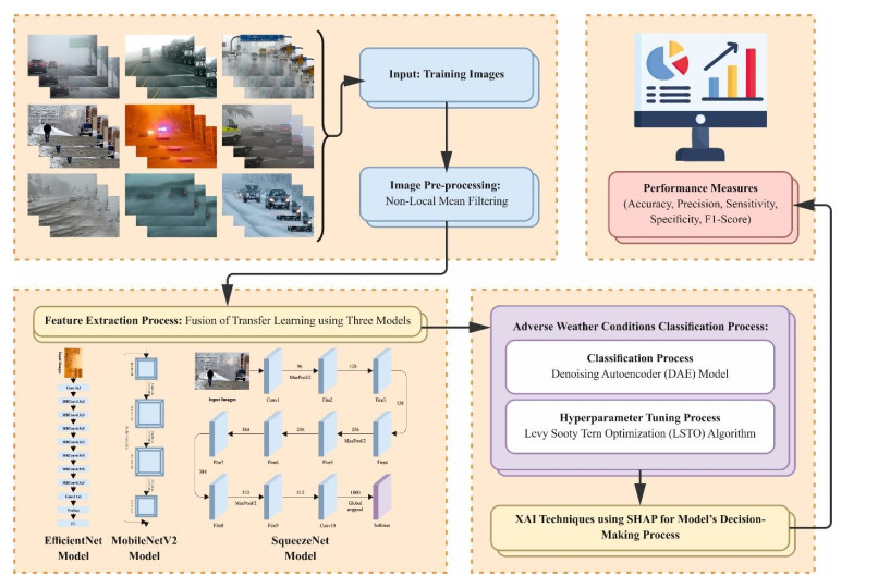
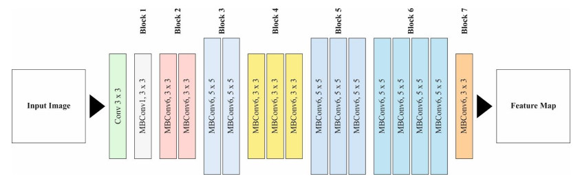
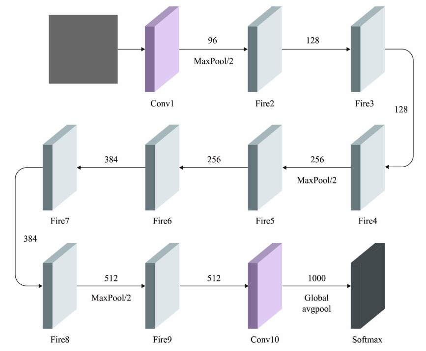
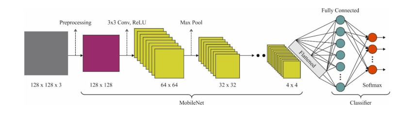
Autonomous vehicles (AVs), particularly self-driving cars, have produced a large amount of interest in artificial intelligence (AI), intelligent transportation, and computer vision. Tracing and detecting numerous targets in real-time, mainly in city arrangements in adversarial environmental conditions, has become a significant challenge for AVs. The effectiveness of vehicle detection has been measured as a crucial stage in intelligent visual surveillance or traffic monitoring. After developing driver assistance and AV methods, adversarial weather conditions have become an essential problem. Nowadays, deep learning (DL) and machine learning (ML) models are critical to enhancing object detection in AVs, particularly in adversarial weather conditions. However, according to statistical learning, conventional AI is fundamental, facing restrictions due to manual feature engineering and restricted flexibility in adaptive environments. This study presents the explainable artificial intelligence with fusion-based transfer learning on adverse weather conditions detection for autonomous vehicles (XAIFTL-AWCDAV) method. The XAIFTL-AWCDAV model's main aim is to detect and classify weather conditions for AVs in challenging scenarios. In the preprocessing stage, the XAIFTL-AWCDAV model utilizes a non-local mean filtering (NLM) method for noise reduction. Besides, the XAIFTL-AWCDAV model performs feature extraction by fusing three models: EfficientNet, SqueezeNet, and MobileNetv2. The denoising autoencoder (DAE) technique is employed to classify adverse weather conditions. Next, the DAE method's hyperparameter selection uses the Levy sooty tern optimization (LSTO) approach. Finally, to ensure the transparency of the model's predictions, XAIFTL-AWCDAV integrates explainable AI (XAI) techniques, utilizing SHAP to visualize and interpret each feature's impact on the model's decision-making process. The efficiency of the XAIFTL-AWCDAV method is validated by comprehensive studies using a benchmark dataset. Numerical results show that the XAIFTL-AWCDAV method obtained a superior value of 98.90% over recent techniques.
Citation: Khaled Tarmissi, Hanan Abdullah Mengash, Noha Negm, Yahia Said, Ali M. Al-Sharafi. Explainable artificial intelligence with fusion-based transfer learning on adverse weather conditions detection using complex data for autonomous vehicles[J]. AIMS Mathematics, 2024, 9(12): 35678-35701. doi: 10.3934/math.20241693
Autonomous vehicles (AVs), particularly self-driving cars, have produced a large amount of interest in artificial intelligence (AI), intelligent transportation, and computer vision. Tracing and detecting numerous targets in real-time, mainly in city arrangements in adversarial environmental conditions, has become a significant challenge for AVs. The effectiveness of vehicle detection has been measured as a crucial stage in intelligent visual surveillance or traffic monitoring. After developing driver assistance and AV methods, adversarial weather conditions have become an essential problem. Nowadays, deep learning (DL) and machine learning (ML) models are critical to enhancing object detection in AVs, particularly in adversarial weather conditions. However, according to statistical learning, conventional AI is fundamental, facing restrictions due to manual feature engineering and restricted flexibility in adaptive environments. This study presents the explainable artificial intelligence with fusion-based transfer learning on adverse weather conditions detection for autonomous vehicles (XAIFTL-AWCDAV) method. The XAIFTL-AWCDAV model's main aim is to detect and classify weather conditions for AVs in challenging scenarios. In the preprocessing stage, the XAIFTL-AWCDAV model utilizes a non-local mean filtering (NLM) method for noise reduction. Besides, the XAIFTL-AWCDAV model performs feature extraction by fusing three models: EfficientNet, SqueezeNet, and MobileNetv2. The denoising autoencoder (DAE) technique is employed to classify adverse weather conditions. Next, the DAE method's hyperparameter selection uses the Levy sooty tern optimization (LSTO) approach. Finally, to ensure the transparency of the model's predictions, XAIFTL-AWCDAV integrates explainable AI (XAI) techniques, utilizing SHAP to visualize and interpret each feature's impact on the model's decision-making process. The efficiency of the XAIFTL-AWCDAV method is validated by comprehensive studies using a benchmark dataset. Numerical results show that the XAIFTL-AWCDAV method obtained a superior value of 98.90% over recent techniques.

| [1] |
M. Hassaballah, M. A. Kenk, K. Muhammad, S. Minaee, Vehicle detection and tracking in adverse weather using a deep learning framework, IEEE Trans. Intell. Transp. Syst., 22 (2020), 4230–4242. https://doi.org/10.1109/TITS.2020.3014013 doi: 10.1109/TITS.2020.3014013

|
| [2] | M. A. Kenk, M. Hassaballah, DAWN: Vehicle detection in adverse weather nature dataset, arXiv preprint, 2020. |
| [3] |
D. Wang, J. G. Wang, K. Xu, Deep learning for object detection, classification and tracking in industry applications, Sensors, 21 (2021), 7349. https://doi.org/10.3390/s21217349 doi: 10.3390/s21217349
|
| [4] |
J. Vargas, S. Alsweiss, O. Toker, R. Razdan, J. Santos, An overview of autonomous vehicles sensors and their vulnerability to weather conditions, Sensors, 21 (2021), 5397. https://doi.org/10.3390/s21165397 doi: 10.3390/s21165397
|
| [5] |
Y. Zhang, A. Carballo, H. Yang, K. Takeda, Perception and sensing for autonomous vehicles under adverse weather conditions: A survey, ISPRS J. Photogramm., 196 (2023), 146−177. https://doi.org/10.1016/j.isprsjprs.2022.12.021 doi: 10.1016/j.isprsjprs.2022.12.021
|
| [6] | A. Balasubramaniam, S. Pasricha, Object detection in autonomous vehicles: Status and open challenges, arXiv preprint, 2022. |
| [7] | A. Z. Abualkishik, R. Almajed, W. Thompson, Multi-attribute decision-making method for prioritizing autonomous vehicles in real-time traffic management: Towards active sustainable transport, Int. J. Wirel. Ad Hoc Commun., 3 (2021), 91−101. https://doi.org/10.54216/IJWAC.030204 |
| [8] |
A. S. Mohammed, A. Amamou, F. K. Ayevide, S. Kelouwani, K. Agbossou, N. Zioui, The perception system of intelligent ground vehicles in all weather conditions: A systematic literature review, Sensors, 20 (2020), 6532. https://doi.org/10.3390/s20226532 doi: 10.3390/s20226532
|
| [9] | J. Li, R. Xu, J. Ma, Q. Zou, J. Ma, H. Yu, Domain adaptive object detection for autonomous driving under foggy weather, In: Proceedings of the IEEE/CVF Winter Conference on Applications of Computer Vision, 2023,612−622. https://doi.org/10.1109/WACV56688.2023.00068 |
| [10] |
M. Hasanujjaman, M. Z. Chowdhury, M. T. Hossan, Y. M. Jang, Autonomous vehicle driving in harsh weather: Adaptive fusion alignment modeling and analysis, Arab. J. Sci. Eng., 49 (2024), 6631−6640. https://doi.org/10.1007/s13369-023-08389-1 doi: 10.1007/s13369-023-08389-1
|
| [11] |
E. Q. Appiah, S. Mensah, Object detection in adverse weather conditions for autonomous vehicles, Multimed. Tools Appl., 83 (2024), 28235−28261. https://doi.org/10.1007/s11042-023-16453-z doi: 10.1007/s11042-023-16453-z
|
| [12] | N. U. A. Tahir, Z. Zhang, M. Asim, J. Chen, M. El Affendi, Object detection in autonomous vehicles under adverse weather: A review of traditional and deep learning approaches, Algorithms, 17 (2024), 103. https://doi.org/10.3390/a17030103 |
| [13] |
A. Vellaidurai, M. Rathinam, A novel oyolov5 model for vehicle detection and classification in adverse weather conditions, Multimed. Tools Appl., 83 (2024), 25037−25054. https://doi.org/10.1007/s11042-023-16450-2 doi: 10.1007/s11042-023-16450-2
|
| [14] |
M. Carvalho, S. Moradi, F. Hosseinnouri, K. Keshavan, E. Villeneuve, I. Gultepe, et al., Towards a model of snow accretion for autonomous vehicles, Atmosphere, 15 (2024), 548. https://doi.org/10.3390/atmos15050548 doi: 10.3390/atmos15050548
|
| [15] |
L. Wen, Y. Peng, M. Lin, N. Gan, R. Tan, Multi-modal contrastive learning for LiDAR point cloud rail-obstacle detection in complex weather, Electronics, 13 (2024), 220. https://doi.org/10.3390/electronics13010220 doi: 10.3390/electronics13010220
|
| [16] |
Z. Zhu, X. Li, J. Zhai, H. Hu, PODB: A learning-based polarimetric object detection benchmark for road scenes in adverse weather conditions, Inform. Fusion, 108 (2024), 102385. https://doi.org/10.1016/j.inffus.2024.102385 doi: 10.1016/j.inffus.2024.102385
|
| [17] | M. Kondapally, K. N. Kumar, C. Vishnu, C. K. Mohan, Towards a transitional weather scene recognition approach for autonomous vehicles, IEEE T. Intell. Transp., 2023. https://doi.org/10.1109/TITS.2023.3331882 |
| [18] |
G. Hou, Evaluating efficiency and safety of mixed traffic with connected and autonomous vehicles in adverse weather, Sustainability, 15 (2023), 3138. https://doi.org/10.3390/su15043138 doi: 10.3390/su15043138
|
| [19] |
Z. Chen, H. Zeng, Y. Wang, W. Yang, Y. Guan, W. Liu, A texture enhancement method for oceanic internal wave synthetic aperture radar images based on non-local mean filtering and texture layer enhancement, Remote Sens., 16 (2024), 1172. https://doi.org/10.3390/rs16071172 doi: 10.3390/rs16071172
|
| [20] |
G. M. S. Himel, M. M. Islam, M. Rahaman, Utilizing EfficientNet for sheep breed identification in low-resolution images, Syst. Soft Comput., 6 (2024), 200093. https://doi.org/10.1016/j.sasc.2024.200093 doi: 10.1016/j.sasc.2024.200093
|
| [21] |
S. Singh, P. K. Jain, N. Sharma, M. Pohit, S. Roy, Atherosclerotic plaque classification in carotid ultrasound images using machine learning and explainable deep learning, Intel. Med., 4 (2024), 83−95. https://doi.org/10.1016/j.imed.2023.05.003 doi: 10.1016/j.imed.2023.05.003
|
| [22] | G. Zhou, Q. He, X. Liu, X. Kai, W. Cao, J. Ding, et al., Optimizing MobileNetV2 for improved accuracy in early gastric cancer detection based on dynamic pelican optimizer, Heliyon, 10 (2024). https://doi.org/10.1016/j.heliyon.2024.e35854 |
| [23] |
R. Ramakotti, S. Paneerselvam, An architecture-oriented analysis of stacked denoising autoencoders, Proc. Comput. Sci., 235 (2024), 2154−2166. https://doi.org/10.1016/j.procs.2024.04.204 doi: 10.1016/j.procs.2024.04.204
|
| [24] |
J. Zhang, Levy sooty tern optimization algorithm builds DNA storage coding sets for random access, Entropy, 26 (2024), 778. https://doi.org/10.3390/e26090778 doi: 10.3390/e26090778
|
| [25] |
A. M. Salih, Z. Raisi‐Estabragh, I. B. Galazzo, P. Radeva, S. E. Petersen, K. Lekadir, et al., A perspective on explainable artificial intelligence methods: SHAP and LIME, Adv. Intell. Syst., 2024. https://doi.org/10.1002/aisy.202400304 doi: 10.1002/aisy.202400304
|
| [26] |
J. Ukwaththa, S. Herath, D. P. P. Meddage, A review of machine learning (ML) and explainable artificial intelligence (XAI) methods in additive manufacturing (3D printing), Mater. Today Commun., 2024. https://doi.org/10.1016/j.mtcomm.2024.110294 doi: 10.1016/j.mtcomm.2024.110294
|
| [27] |
D. P. P. Meddage, I. Fonseka, D. Mohotti, K. Wijesooriya, C. K. Lee, An explainable machine learning approach to predict the compressive strength of graphene oxide-based concrete, Constr. Build. Mater., 449 (2024), 138346. https://doi.org/10.1016/j.conbuildmat.2024.138346 doi: 10.1016/j.conbuildmat.2024.138346
|
| [28] | https://data.mendeley.com/datasets/766ygrbt8y/3 |
| [29] |
Q. A. Al-Haija, M. Gharaibeh, A. Odeh, Detection in adverse weather conditions for autonomous vehicles via deep learning, Ai, 3 (2022), 303−317. https://doi.org/10.3390/ai3020019 doi: 10.3390/ai3020019
|
| [30] |
M. N. Khan, M. M. Ahmed, Weather and surface condition detection based on road-side webcams: Application of pre-trained convolutional neural network, Int. J. Transp. Sci. Tec., 11 (2022), 468−483. https://doi.org/10.1016/j.ijtst.2021.06.003 doi: 10.1016/j.ijtst.2021.06.003
|
Figures(12) / Tables(4)

Khaled Tarmissi, Hanan Abdullah Mengash, Noha Negm, Yahia Said, Ali M. Al-Sharafi. Explainable artificial intelligence with fusion-based transfer learning on adverse weather conditions detection using complex data for autonomous vehicles[J]. AIMS Mathematics, 2024, 9(12): 35678-35701. doi: 10.3934/math.20241693


 DownLoad: