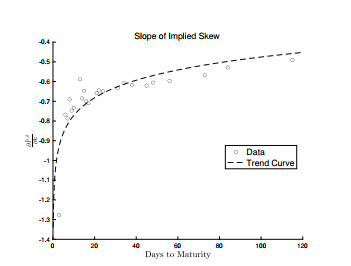
In this paper, we proposed a stochastic volatility model in which the volatility was given by stochastic processes representing two characteristic time scales of variation driven by approximate fractional Brownian motions with two Hurst exponents. We obtained an approximate closed-form formula for a European vanilla option price and the corresponding implied volatility formula based on singular and regular perturbations and a Mellin transform. The explicit formula for the implied volatility allowed us to find the slope of the implied volatility skew with respect to the Hurst exponent and time-to-maturity. The proposed model allows the market volatility behavior to be captured uniformly in time-to-maturity. We conducted an empirical analysis to find the validity of the proposed model by comparing it with other models and Monte Carlo simulation. Further, we extended the pricing result for the vanilla option to two path-dependent exotic (barrier and lookback) options and obtained the corresponding price formulas explicitly.
Citation: Min-Ku Lee, Jeong-Hoon Kim. Pricing vanilla, barrier, and lookback options under two-scale stochastic volatility driven by two approximate fractional Brownian motions[J]. AIMS Mathematics, 2024, 9(9): 25545-25576. doi: 10.3934/math.20241248
In this paper, we proposed a stochastic volatility model in which the volatility was given by stochastic processes representing two characteristic time scales of variation driven by approximate fractional Brownian motions with two Hurst exponents. We obtained an approximate closed-form formula for a European vanilla option price and the corresponding implied volatility formula based on singular and regular perturbations and a Mellin transform. The explicit formula for the implied volatility allowed us to find the slope of the implied volatility skew with respect to the Hurst exponent and time-to-maturity. The proposed model allows the market volatility behavior to be captured uniformly in time-to-maturity. We conducted an empirical analysis to find the validity of the proposed model by comparing it with other models and Monte Carlo simulation. Further, we extended the pricing result for the vanilla option to two path-dependent exotic (barrier and lookback) options and obtained the corresponding price formulas explicitly.

| [1] |
E. Alòs, R. De Santiago, J. Vives, Calibration of stochastic volatility models via second order approximation: The Heston case, Int. J. Theor. Appl. Fin., 18 (2016), 1550036. https://doi.org/10.1142/S0219024915500363 doi: 10.1142/S0219024915500363

|
| [2] |
E. Alòs, J. A. Leon, J. Vives, On the short-time behavior of the implied volatility for jump-diffusion models with stochastic volatility, Financ. Stoch., 11 (2007), 571–589. https://doi.org/10.1007/s00780-007-0049-1 doi: 10.1007/s00780-007-0049-1
|
| [3] |
E. Alòs, J. A. Leon, An intuitive introduction to fractional and rough volatilities, Mathematics, 9 (2021), 994. https://doi.org/10.3390/math9090994 doi: 10.3390/math9090994
|
| [4] |
C. Bayer, P. Friz, J. Gatheral, Pricing under rough volatility, Quant. Financ., 16 (2016), 887–904. https://doi.org/10.1080/14697688.2015.1099717 doi: 10.1080/14697688.2015.1099717
|
| [5] |
M. Bennedsen, A. Lunde, M. S. Pakkanen, Decoupling the short-and long-term behavior of stochastic volatility, J. Financ. Economet., 20 (2022), 961–1006. https://doi.org/10.1093/jjfinec/nbaa049 doi: 10.1093/jjfinec/nbaa049
|
| [6] | F. Black, M. Scholes, The pricing of options and corporate liabilities, J. Polit. Econ., 81 (1973), 637–654. |
| [7] | Y. Chang, Y. Wang, S. Zhang, Option pricing under double Heston model with approximative fractional stochastic volatility, Math. Probl. Eng., 2021 (2021), 6634779. |
| [8] |
P. Cheridito, Mixed fractional Brownian motion, Bernoulli, 7 (2001), 913–934. https://doi.org/10.2307/3318626 doi: 10.2307/3318626
|
| [9] |
F. Comte, E. Renault, Long memory in continuous-time stochastic volatility models, Math. Financ., 8 (1998), 291–323. https://doi.org/10.1111/1467-9965.00057 doi: 10.1111/1467-9965.00057
|
| [10] |
R. Cont, P. Das, Rough volatility: Fact or artefact? Sankhya B, 86 (2024), 191–223. https://doi.org/10.1007/s13571-024-00322-2 doi: 10.1007/s13571-024-00322-2
|
| [11] |
N. T. Dung, Semimartingale approximation of fractional Brownian motion and its applications, Comput. Math. Appl., 61 (2011), 1844–1854. https://doi.org/10.1016/j.camwa.2011.02.013 doi: 10.1016/j.camwa.2011.02.013
|
| [12] |
M. Forde, H. Zhang, Asymptotics for rough stochastic volatility models, SIAM J. Financ. Math., 8 (2017), 114–145. https://doi.org/10.1137/15M1009330 doi: 10.1137/15M1009330
|
| [13] |
J. P. Fouque, M. Lorig, R. Sircar, Second order multiscale stochastic volatility asymptotics: Stochastic terminal layer analysis & calibration, Financ. Stoch., 20 (2016), 543–588. https://doi.org/10.1007/s00780-016-0298-y doi: 10.1007/s00780-016-0298-y
|
| [14] |
J. P. Fouque, G. Papanicolaou, R. Sircar, K. Sølna, Multiscale stochastic volatility asymptotics, SIAM J. Multiscale Model. Simul., 2 (2003), 22–42. https://doi.org/10.1137/030600291 doi: 10.1137/030600291
|
| [15] | J. P. Fouque, G. Papanicolaou, R. Sircar, K. Sølna, Multiscale stochastic volatility for equity, interest rate and credit derivatives, Cambridge University Press, Cambridge, England, 2011. |
| [16] |
M. Fukasawa, J. Gatheral, A rough SABR formula, Front. Math. Financ., 1 (2022), 81–97. https://doi.org/10.3934/fmf.2021003 doi: 10.3934/fmf.2021003
|
| [17] |
J. Garnier, K. Solna, Correction to Black-Scholes formula due to fractional stochastic volatility, SIAM J. Financ. Math., 8 (2017), 560–588. https://doi.org/10.1137/15M1036749 doi: 10.1137/15M1036749
|
| [18] | J. Gatheral, Consistent modeling of SPX and VIX options, The Fifth World Congress of the Bachelier Finance Society London, July 18, 2008. |
| [19] |
J. Gatheral, T. Jaisson, M. Rosenbaum, Volatility is rough, Quant. Financ., 18 (2018), 933–949. https://doi.org/10.1080/14697688.2017.1393551 doi: 10.1080/14697688.2017.1393551
|
| [20] |
H. Guennoun, A. Jacquier, P. Roome, F. Shi, Asymptotic behavior of the fractional Heston model, SIAM J. Financ. Math., 9 (2018), 1017–1045. https://doi.org/10.1137/17M1142892 doi: 10.1137/17M1142892
|
| [21] |
H. G. Kim, S. J. Kwon, J. H. Kim, Fractional stochasic volatility correction to CEV implied volatility, Quant. Financ., 21 (2021), 565–574. https://doi.org/10.1080/14697688.2020.1812703 doi: 10.1080/14697688.2020.1812703
|
| [22] |
B. Mandelbrot, J. van Ness, Fractional Brownian motions, fractional noises and applications, SIAM Rev., 10 (1968), 422–437. https://doi.org/10.1137/1010093 doi: 10.1137/1010093
|
| [23] | B. Oksendal, Stochastic differential equations: An introduction with applications, Springer, Heidelberg, 2013. |
| [24] |
G. Pang, M. S. Taqqu, Nonstationary self-similar Gaussian processes as scaling limits of power-law shot noise processes and generalizations of fractional Brownian motion, High Frequency, 2 (2019), 95–112. https://doi.org/10.1002/hf2.10028 doi: 10.1002/hf2.10028
|
| [25] | A. Pascucci, PDE and martingale methods in option pricing, Berlin, Springer-Verlag, 2011. |
| [26] |
J. Pospisil, T. Sobotka, Market calibration under a long memory stochastic volatility model, Appl. Math. Financ., 23 (2016), 323–343. https://doi.org/10.1080/1350486X.2017.1279977 doi: 10.1080/1350486X.2017.1279977
|
| [27] | A. D. Polyanin, V. E. Nazaikinskii, Handbook of linear partial differential equations for engineers and scientists, Chapman and Hall/CRC, New York, 2016. https://doi.org/10.1201/b19056 |
| [28] |
L. C. G. Rogers, Arbitrage with fractional Brownian motion, Math. Financ., 7 (1997), 95–105. https://doi.org/10.1111/1467-9965.00025 doi: 10.1111/1467-9965.00025
|
| [29] |
P. Sattayatham, A. Intarasit, An approximate formula of European option for fractional stochastic volatility jump-diffusion model, Math. Stat., 7 (2011), 230–238. https://doi.org/10.3844/jmssp.2011.230.238 doi: 10.3844/jmssp.2011.230.238
|
| [30] |
S. Shi, J. Yu, Volatility puzzle: Long memory or antipersistency, Manag. Sci., 69 (2023), 3861–3883. https://doi.org/10.1287/mnsc.2022.4552 doi: 10.1287/mnsc.2022.4552
|
| [31] | S. Shreve, Stochastic calculus for finance Ⅱ: Continuous-time models, Springer, Heidelberg, 2004. |
| [32] |
T. H. Thao, An approximate approach to fractional analysis for finance, Nonlinear Anal.-Real, 7 (2006), 124–132. https://doi.org/10.1016/j.nonrwa.2004.08.012 doi: 10.1016/j.nonrwa.2004.08.012
|
| [33] |
X. Wang, W. Xiao, J. Yu, Modeling and forecasting realized volatility with the fractional Ornstein-Uhlenbeck process, J. Econometrics, 232 (2023), 389–415. https://doi.org/10.1016/j.jeconom.2021.08.001 doi: 10.1016/j.jeconom.2021.08.001
|
| [34] | P. Wilmott, Paul Wilmott on quantitative finance, Wiley, West Sussex, England, 2006. |
| [35] |
W. Xiao, J. Yu, Asymptotic theory for estimating drift parameters in the fractional Vasicek model, Economet. Theor., 35 (2019), 198–231. https://doi.org/10.1017/S0266466618000051 doi: 10.1017/S0266466618000051
|
| [36] |
W. Xiao, J. Yu, Asymptotic theory for rough fractional Vasicek models, Econ. Lett., 177 (2019), 26–29. https://doi.org/10.1016/j.econlet.2019.01.020 doi: 10.1016/j.econlet.2019.01.020
|


Figures(4) / Tables(5)

Min-Ku Lee, Jeong-Hoon Kim. Pricing vanilla, barrier, and lookback options under two-scale stochastic volatility driven by two approximate fractional Brownian motions[J]. AIMS Mathematics, 2024, 9(9): 25545-25576. doi: 10.3934/math.20241248


 DownLoad: