The (2+1)-dimensional Chaffee-Infante equation (CIE) is a significant model of the ion-acoustic waves in plasma. The primary objective of this paper was to establish and examine closed-form soliton solutions to the CIE using the modified extended direct algebraic method (m-EDAM), a mathematical technique. By using a variable transformation to convert CIE into a nonlinear ordinary differential equation (NODE), which was then reduced to a system of nonlinear algebraic equations with the assumption of a closed-form solution, the strategic m-EDAM was implemented. When the resulting problem was solved using the Maple tool, many soliton solutions in the shapes of rational, exponential, trigonometric, and hyperbolic functions were produced. By using illustrated 3D and density plots to evaluate several soliton solutions for the provided definite values of the parameters, it was possible to determine if the soliton solutions produced for CIE are cuspon or kink solitons. Additionally, it has been shown that the m-EDAM is a robust, useful, and user-friendly instrument that provides extra generic wave solutions for nonlinear models in mathematical physics and engineering.
Citation: Naveed Iqbal, Muhammad Bilal Riaz, Meshari Alesemi, Taher S. Hassan, Ali M. Mahnashi, Ahmad Shafee. Reliable analysis for obtaining exact soliton solutions of (2+1)-dimensional Chaffee-Infante equation[J]. AIMS Mathematics, 2024, 9(6): 16666-16686. doi: 10.3934/math.2024808
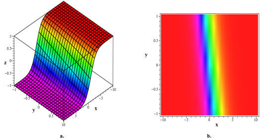
The (2+1)-dimensional Chaffee-Infante equation (CIE) is a significant model of the ion-acoustic waves in plasma. The primary objective of this paper was to establish and examine closed-form soliton solutions to the CIE using the modified extended direct algebraic method (m-EDAM), a mathematical technique. By using a variable transformation to convert CIE into a nonlinear ordinary differential equation (NODE), which was then reduced to a system of nonlinear algebraic equations with the assumption of a closed-form solution, the strategic m-EDAM was implemented. When the resulting problem was solved using the Maple tool, many soliton solutions in the shapes of rational, exponential, trigonometric, and hyperbolic functions were produced. By using illustrated 3D and density plots to evaluate several soliton solutions for the provided definite values of the parameters, it was possible to determine if the soliton solutions produced for CIE are cuspon or kink solitons. Additionally, it has been shown that the m-EDAM is a robust, useful, and user-friendly instrument that provides extra generic wave solutions for nonlinear models in mathematical physics and engineering.

| [1] |
A. Seadawy, A. Sayed, Soliton solutions of cubic-quintic nonlinear Schrödinger and variant Boussinesq equations by the first integral method, Filomat, 31 (2017), 4199–4208. http://dx.doi.org/10.2298/FIL1713199S doi: 10.2298/FIL1713199S

|
| [2] |
H. Yasmin, A. Alshehry, A. Ganie, A. Mahnashi, R. Shah, Perturbed Gerdjikov-Ivanov equation: soliton solutions via Backlund transformation, Optik, 298 (2024), 171576. http://dx.doi.org/10.1016/j.ijleo.2023.171576 doi: 10.1016/j.ijleo.2023.171576
|
| [3] |
A. Jawad, M. Petkovi, A. Biswas, Modified simple equation method for nonlinear evolution equations, Appl. Math. Comput., 217 (2010), 869–877. http://dx.doi.org/10.1016/j.amc.2010.06.030 doi: 10.1016/j.amc.2010.06.030
|
| [4] |
H. Khan, Shoaib, D. Baleanu, P. Kumam, J. Al-Zaidy, Families of travelling waves solutions for fractional-order extended shallow water wave equations, using an innovative analytical method, IEEE Access, 7 (2019), 107523–107532. http://dx.doi.org/10.1109/ACCESS.2019.2933188 doi: 10.1109/ACCESS.2019.2933188
|
| [5] |
H. Khan, S. Barak, P. Kumam, M. Arif, Analytical solutions of fractional Klein-Gordon and gas dynamics equations, via the (G'/G)-expansion method, Symmetry, 11 (2019), 566. http://dx.doi.org/10.3390/sym11040566 doi: 10.3390/sym11040566
|
| [6] |
H. Khan, R. Shah, J. Gomez-Aguilar, Shoaib, D. Baleanu, P. Kumam, Travelling waves solution for fractional-order biological population model, Math. Model. Nat. Phenom., 16 (2021), 32. http://dx.doi.org/10.1051/mmnp/2021016 doi: 10.1051/mmnp/2021016
|
| [7] |
K. Nisar, O. Ilhan, S. Abdulazeez, J. Manafian, S. Mohammed, M. Osman, Novel multiple soliton solutions for some nonlinear PDEs via multiple Exp-function method, Results Phys., 21 (2021), 103769. http://dx.doi.org/10.1016/j.rinp.2020.103769 doi: 10.1016/j.rinp.2020.103769
|
| [8] |
E. Yusufolu, A. Bekir, Solitons and periodic solutions of coupled nonlinear evolution equations by using the sine-cosine method, Int. J. Comput. Math., 83 (2006), 915–924. http://dx.doi.org/10.1080/00207160601138756 doi: 10.1080/00207160601138756
|
| [9] |
E. Fan, H. Zhang, A note on the homogeneous balance method, Phys. Lett. A, 246 (1998), 403–406. http://dx.doi.org/10.1016/S0375-9601(98)00547-7 doi: 10.1016/S0375-9601(98)00547-7
|
| [10] |
Z. Rahman, M. Zulfikar Ali, H. Roshid, Closed-form soliton solutions of three nonlinear fractional models through proposed improved Kudryashov method, Chinese Phys. B, 30 (2021), 050202. http://dx.doi.org/10.1088/1674-1056/abd165 doi: 10.1088/1674-1056/abd165
|
| [11] |
M. Ozisik, A. Secer, M. Bayram, On solitary wave solutions for the extended nonlinear Schrödinger equation via the modified F-expansion method, Opt. Quant. Electron., 55 (2023), 215. http://dx.doi.org/10.1007/s11082-022-04476-z doi: 10.1007/s11082-022-04476-z
|
| [12] |
Z. Lan, S. Dong, B. Gao, Y. Shen, Bilinear form and soliton solutions for a higher order wave equation, Appl. Math. Lett., 134 (2022), 108340. http://dx.doi.org/10.1016/j.aml.2022.108340 doi: 10.1016/j.aml.2022.108340
|
| [13] |
H. Hussein, H. Ahmed, W. Alexan, Analytical soliton solutions for cubic-quartic perturbations of the Lakshmanan-Porsezian-Daniel equation using the modified extended tanh function method, Ain Shams Eng. J., 15 (2024), 102513. http://dx.doi.org/10.1016/j.asej.2023.102513 doi: 10.1016/j.asej.2023.102513
|
| [14] |
G. Akram, M. Sadaf, S. Arshed, F. Sameen, Bright, dark, kink, singular and periodic soliton solutions of Lakshmanan-Porsezian-Daniel model by generalized projective Riccati equations method, Optik, 241 (2021), 167051. http://dx.doi.org/10.1016/j.ijleo.2021.167051 doi: 10.1016/j.ijleo.2021.167051
|
| [15] |
L. Li, E. Li, M. Wang, The (G'/G, 1/G)-expansion method and its application to travelling wave solutions of the Zakharov equations, Appl. Math. J. Chin. Univ., 25 (2010), 454–462. http://dx.doi.org/10.1007/s11766-010-2128-x doi: 10.1007/s11766-010-2128-x
|
| [16] |
X. Yang, Z. Deng, Y. Wei, A Riccati-Bernoulli sub-ODE method for nonlinear partial differential equations and its application, Adv. Differ. Equ., 2015 (2015), 117. http://dx.doi.org/10.1186/s13662-015-0452-4 doi: 10.1186/s13662-015-0452-4
|
| [17] |
S. Dai, Poincare-Lighthill-Kuo method and symbolic computation, Appl. Math. Mech., 22 (2001), 261–269. http://dx.doi.org/10.1007/BF02437964 doi: 10.1007/BF02437964
|
| [18] |
H. Durur, A. Kurt, O. Tasbozan, New travelling wave solutions for KdV6 equation using sub equation method, Applied Mathematics and Nonlinear Sciences, 5 (2020), 455–460. http://dx.doi.org/10.2478/amns.2020.1.00043 doi: 10.2478/amns.2020.1.00043
|
| [19] |
S. Bibi, S. Mohyud-Din, U. Khan, N. Ahmed, Khater method for nonlinear Sharma Tasso-Olever (STO) equation of fractional order, Results Phys., 7 (2017), 4440–4450. http://dx.doi.org/10.1016/j.rinp.2017.11.008 doi: 10.1016/j.rinp.2017.11.008
|
| [20] |
H. Ur Rehman, R. Akber, A. Wazwaz, H. Alshehri, M. Osman, Analysis of Brownian motion in stochastic Schrödinger wave equation using Sardar sub-equation method, Optik, 289 (2023), 171305. http://dx.doi.org/10.1016/j.ijleo.2023.171305 doi: 10.1016/j.ijleo.2023.171305
|
| [21] |
M. Alqhtani, K. Saad, R. Shah, W. Hamanah, Discovering novel soliton solutions for (3+1)-modified fractional Zakharov-Kuznetsov equation in electrical engineering through an analytical approach, Opt. Quant. Electron., 55 (2023), 1149. http://dx.doi.org/10.1007/s11082-023-05407-2 doi: 10.1007/s11082-023-05407-2
|
| [22] |
M. Al-Sawalha, S. Mukhtar, R. Shah, A. Ganie, K. Moaddy, Solitary waves propagation analysis in nonlinear dynamical system of fractional coupled Boussinesq-Whitham-Broer-Kaup equation, Fractal Fract., 7 (2023), 889. http://dx.doi.org/10.3390/fractalfract7120889 doi: 10.3390/fractalfract7120889
|
| [23] |
H. Yasmin, A. Alshehry, A. Ganie, A. Shafee, R. Shah, Noise effect on soliton phenomena in fractional stochastic Kraenkel-Manna-Merle system arising in ferromagnetic materials, Sci. Rep., 14 (2024), 1810. http://dx.doi.org/10.1038/s41598-024-52211-3 doi: 10.1038/s41598-024-52211-3
|
| [24] |
H. Yasmin, N. Aljahdaly, A. Saeed, R. Shah, Investigating symmetric soliton solutions for the fractional coupled Konno-Onno system using improved versions of a novel analytical technique, Mathematics, 11 (2023), 2686. http://dx.doi.org/10.3390/math11122686 doi: 10.3390/math11122686
|
| [25] |
S. El-Tantawy, H. Alyousef, R. Matoog, R. Shah, On the optical soliton solutions to the fractional complex structured (1+1)-dimensional perturbed Gerdjikov-Ivanov equation, Phys. Scr., 99 (2024), 035249. http://dx.doi.org/10.1088/1402-4896/ad241b doi: 10.1088/1402-4896/ad241b
|
| [26] |
L. Li, C. Duan, F. Yu, An improved Hirota bilinear method and new application for a nonlocal integrable complex modified Korteweg-de Vries (MKdV) equation, Phys. Lett. A, 383 (2019), 1578–1582. http://dx.doi.org/10.1016/j.physleta.2019.02.031 doi: 10.1016/j.physleta.2019.02.031
|
| [27] |
T. Han, Y. Jiang, Bifurcation, chaotic pattern and traveling wave solutions for the fractional Bogoyavlenskii equation with multiplicative noise, Phys. Scr., 99 (2024), 035207. http://dx.doi.org/10.1088/1402-4896/ad21ca doi: 10.1088/1402-4896/ad21ca
|
| [28] |
T. Han, Y. Jiang, J. Lyu, Chaotic behavior and optical soliton for the concatenated model arising in optical communication, Results Phys., 58 (2024), 107467. http://dx.doi.org/10.1016/j.rinp.2024.107467 doi: 10.1016/j.rinp.2024.107467
|
| [29] |
R. Ali, E. Tag-eldin, A comparative analysis of generalized and extended (G'/G)-Expansion methods for travelling wave solutions of fractional Maccari's system with complex structure, Alex. Eng. J., 79 (2023), 508–530. http://dx.doi.org/10.1016/j.aej.2023.08.007 doi: 10.1016/j.aej.2023.08.007
|
| [30] |
R. Ali, A. Hendy, M. Ali, A. Hassan, F. Awwad, E. Ismail, Exploring propagating soliton solutions for the fractional Kudryashov-Sinelshchikov equation in a mixture of liquid-gas bubbles under the consideration of heat transfer and viscosity, Fractal Fract., 7 (2023), 773. http://dx.doi.org/10.3390/fractalfract7110773 doi: 10.3390/fractalfract7110773
|
| [31] |
Y. Shi, C. Song, Y. Chen, H. Rao, T. Yang, Complex standard eigenvalue problem derivative computation for Laminar-Turbulent transition prediction, AIAA J., 61 (2023), 3404–3418. http://dx.doi.org/10.2514/1.J062212 doi: 10.2514/1.J062212
|
| [32] |
X. Cai, R. Tang, H. Zhou, Q. Li, S. Ma, D. Wang, et al., Dynamically controlling terahertz wavefronts with cascaded metasurfaces, Advanced Photonics, 3 (2021), 036003. http://dx.doi.org/10.1117/1.AP.3.3.036003 doi: 10.1117/1.AP.3.3.036003
|
| [33] |
A. She, L. Wang, Y. Peng, J. Li, Structural reliability analysis based on improved wolf pack algorithm AK-SS, Structures, 57 (2023), 105289. http://dx.doi.org/10.1016/j.istruc.2023.105289 doi: 10.1016/j.istruc.2023.105289
|
| [34] |
T. Ali, Z. Xiao, H. Jiang, B. Li, A class of digital integrators based on trigonometric quadrature rules, IEEE T. Ind. Electron., 71 (2024), 6128–6138. http://dx.doi.org/10.1109/TIE.2023.3290247 doi: 10.1109/TIE.2023.3290247
|
| [35] |
J. Dong, J. Hu, Y. Zhao, Y. Peng, Opinion formation analysis for expressed and private opinions (EPOs) models: reasoning private opinions from behaviors in group decision-making systems, Expert Syst. Appl., 236 (2024), 121292. http://dx.doi.org/10.1016/j.eswa.2023.121292 doi: 10.1016/j.eswa.2023.121292
|
| [36] |
C. Zhu, M. Al-Dossari, S. Rezapour, S. Shateyi, On the exact soliton solutions and different wave structures to the modified Schrödinger's equation, Results Phys., 54 (2023), 107037. http://dx.doi.org/10.1016/j.rinp.2023.107037 doi: 10.1016/j.rinp.2023.107037
|
| [37] |
C. Zhu, M. Al-Dossari, N. El-Gawaad, S. Alsallami, S. Shateyi, Uncovering diverse soliton solutions in the modified Schrödinger's equation via innovative approaches, Results Phys., 54 (2023), 107100. http://dx.doi.org/10.1016/j.rinp.2023.107100 doi: 10.1016/j.rinp.2023.107100
|
| [38] |
C. Zhu, S. Abdallah, S. Rezapour, S. Shateyi, On new diverse variety analytical optical soliton solutions to the perturbed nonlinear Schrödinger equation, Results Phys., 54 (2023), 107046. http://dx.doi.org/10.1016/j.rinp.2023.107046 doi: 10.1016/j.rinp.2023.107046
|
| [39] |
C. Zhu, S. Idris, M. Abdalla, S. Rezapour, S. Shateyi, B. Gunay, Analytical study of nonlinear models using a modified Schrödinger's equation and logarithmic transformation, Results Phys., 55 (2023), 107183. http://dx.doi.org/10.1016/j.rinp.2023.107183 doi: 10.1016/j.rinp.2023.107183
|
| [40] |
S. Lin, J. Zhang, C. Qiu, Asymptotic analysis for one-stage stochastic linear complementarity problems and applications, Mathematics, 11 (2023), 482. http://dx.doi.org/10.3390/math11020482 doi: 10.3390/math11020482
|
| [41] |
Y. Kai, Z. Yin, On the Gaussian traveling wave solution to a special kind of Schrödinger equation with logarithmic nonlinearity, Mod. Phys. Lett. B, 36 (2022), 2150543. http://dx.doi.org/10.1142/S0217984921505436 doi: 10.1142/S0217984921505436
|
| [42] |
Y. Kai, J. Ji, Z. Yin, Study of the generalization of regularized long-wave equation, Nonlinear Dyn., 107 (2022), 2745–2752. http://dx.doi.org/10.1007/s11071-021-07115-6 doi: 10.1007/s11071-021-07115-6
|
| [43] |
Y. Kai, Z. Yin, Linear structure and soliton molecules of Sharma-Tasso-Olver-Burgers equation, Phys. Lett. A, 452 (2022), 128430. http://dx.doi.org/10.1016/j.physleta.2022.128430 doi: 10.1016/j.physleta.2022.128430
|
| [44] |
S. Noor, A. Alshehry, A. Khan, I. Khan, Analysis of soliton phenomena in (2+1)-dimensional Nizhnik-Novikov-Veselov model via a modified analytical technique, AIMS Mathematics, 8 (2023), 28120–28142. http://dx.doi.org/10.3934/math.20231439 doi: 10.3934/math.20231439
|
| [45] |
I. Ullah, K. Shah, T. Abdeljawad, Study of traveling soliton and fronts phenomena in fractional Kolmogorov-Petrovskii-Piskunov equation, Phys. Scr., 99 (2024), 055259. http://dx.doi.org/10.1088/1402-4896/ad3c7e doi: 10.1088/1402-4896/ad3c7e
|
| [46] |
M. Bilal, J. Iqbal, R. Ali, F. Awwad, E. Ismail, Exploring families of solitary wave solutions for the fractional coupled higgs system using modified extended direct algebraic method, Fractal Fract., 7 (2023), 653. http://dx.doi.org/10.3390/fractalfract7090653 doi: 10.3390/fractalfract7090653
|
| [47] |
R. Ali, Z. Zhang, H. Ahmad, Exploring soliton solutions in nonlinear spatiotemporal fractional quantum mechanics equations: an analytical study, Opt. Quant. Electron., 56 (2024), 838. http://dx.doi.org/10.1007/s11082-024-06370-2 doi: 10.1007/s11082-024-06370-2
|
| [48] |
M. Akbar, N. Ali, J. Hussain, Optical soliton solutions to the (2+1)-dimensional Chaffee-Infante equation and the dimensionless form of the Zakharov equation, Adv. Differ. Equ., 2019 (2019), 446. http://dx.doi.org/10.1186/s13662-019-2377-9 doi: 10.1186/s13662-019-2377-9
|
| [49] |
R. Sakthivel, C. Chun, New soliton solutions of Chaffee-Infante equations using the exp-function method, Z. Naturforsch. A, 65 (2010), 197–202. http://dx.doi.org/10.1515/zna-2010-0307 doi: 10.1515/zna-2010-0307
|
| [50] |
T. Sulaiman, A. Yusuf, M. Alquran, Dynamics of lump solutions to the variable coefficients (2+1)-dimensional Burger's and Chaffee-infante equations, J. Geom. Phys., 168 (2021), 104315. http://dx.doi.org/10.1016/j.geomphys.2021.104315 doi: 10.1016/j.geomphys.2021.104315
|
| [51] |
S. Demiray, U. Bayrakcı, Construction of soliton solutions for Chaffee-Infante equation, AKU J. Sci. Eng., 21 (2021), 1046–1051. http://dx.doi.org/10.35414/akufemubid.946217 doi: 10.35414/akufemubid.946217
|
| [52] |
A. Seadawy, A. Ali, A. Altalbe, A. Bekir, Exact solutions of the (3+1)-generalized fractional nonlinear wave equation with gas bubbles, Sci. Rep., 14 (2024), 1862. http://dx.doi.org/10.1038/s41598-024-52249-3 doi: 10.1038/s41598-024-52249-3
|


Figures(10)

Naveed Iqbal, Muhammad Bilal Riaz, Meshari Alesemi, Taher S. Hassan, Ali M. Mahnashi, Ahmad Shafee. Reliable analysis for obtaining exact soliton solutions of (2+1)-dimensional Chaffee-Infante equation[J]. AIMS Mathematics, 2024, 9(6): 16666-16686. doi: 10.3934/math.2024808


 DownLoad: