A queueing system with the discipline of flexible limited sharing of the server is considered. This discipline assumes the admission, for a simultaneous service, of only a finite number of orders, as well as the use of a reduced service rate when the bandwidth required by the admitted orders is less than the total bandwidth of the server. The orders arrive following a batch-marked Markov arrival process, which is a generalization of the well-known $ MAP $ (Markov arrival process) to the cases of heterogeneous orders and batch arrivals. The orders of different types have different preemptive priorities. The possibility of an increase or a decrease in order priority during the service is suggested to be an effective mechanism to prevent long processing orders from being pushed out of service by just-arrived higher-priority orders. Under a fixed priority scheme and a mechanism of dynamic change of the priorities, the stationary analysis of this queueing system is implemented by considering a suitable multidimensional continuous-time Markov chain with a generator that has an upper Hessenberg structure. The possibility of the optimal restriction on the number of simultaneously serviced orders is numerically demonstrated.
Citation: Alexander Dudin, Sergey Dudin, Rosanna Manzo, Luigi Rarità. Queueing system with batch arrival of heterogeneous orders, flexible limited processor sharing and dynamical change of priorities[J]. AIMS Mathematics, 2024, 9(5): 12144-12169. doi: 10.3934/math.2024593
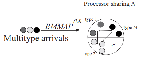
A queueing system with the discipline of flexible limited sharing of the server is considered. This discipline assumes the admission, for a simultaneous service, of only a finite number of orders, as well as the use of a reduced service rate when the bandwidth required by the admitted orders is less than the total bandwidth of the server. The orders arrive following a batch-marked Markov arrival process, which is a generalization of the well-known $ MAP $ (Markov arrival process) to the cases of heterogeneous orders and batch arrivals. The orders of different types have different preemptive priorities. The possibility of an increase or a decrease in order priority during the service is suggested to be an effective mechanism to prevent long processing orders from being pushed out of service by just-arrived higher-priority orders. Under a fixed priority scheme and a mechanism of dynamic change of the priorities, the stationary analysis of this queueing system is implemented by considering a suitable multidimensional continuous-time Markov chain with a generator that has an upper Hessenberg structure. The possibility of the optimal restriction on the number of simultaneously serviced orders is numerically demonstrated.

| [1] |
V. M. Vishnevskii, O. V. Semenova, Mathematical methods to study the polling systems, Autom. Remote. Control, 67 (2006), 173–220. http://dx.doi.org/10.1134/S0005117906020019 doi: 10.1134/S0005117906020019

|
| [2] |
S. Borst, O. Boxma, Polling: past, present, and perspective, Top, 26 (2018), 335–369. http://dx.doi.org/10.1007/s11750-018-0484-5 doi: 10.1007/s11750-018-0484-5
|
| [3] |
V. Vishnevsky, O. Semenova, Polling systems and their application to telecommunication networks, Mathematics, 9 (2021), 117. http://dx.doi.org/10.3390/math9020117 doi: 10.3390/math9020117
|
| [4] |
E. Altman, K. Avrachenkov, U. Ayesta, A survey on discriminatory processor sharing, Queueing Syst., 53 (2006), 53–63. http://dx.doi.org/10.1007/s11134-006-7586-8 doi: 10.1007/s11134-006-7586-8
|
| [5] |
S. F. Yashkov, Processor-sharing queues: some progress in analysis, Queueing Syst., 2 (1987), 1–17. http://dx.doi.org/10.1007/BF01182931 doi: 10.1007/BF01182931
|
| [6] |
S. F. Yashkov, A. S. Yashkova, Processor sharing: a survey of the mathematical theory, Autom. Remote. Control, 68 (2007), 1662–1731. http://dx.doi.org/10.1134/S0005117907090202 doi: 10.1134/S0005117907090202
|
| [7] |
C. D'Apice, A. Dudin, S. Dudin, R. Manzo, Priority queueing system with many types of requests and restricted processor sharing, J. Ambient Intell. Humaniz. Comput., 14 (2023), 12651–12662. http://dx.doi.org/10.1007/s12652-022-04233-w doi: 10.1007/s12652-022-04233-w
|
| [8] |
A. N. Dudin, S. A. Dudin, O. S. Dudina, Analysis of a queueing system with mixed service discipline, Methodol. Comput. Appl. Probab., 25 (2023), 1–19. http://dx.doi.org/10.1007/s11009-023-10042-1 doi: 10.1007/s11009-023-10042-1
|
| [9] |
J. Nair, A. Wierman, B. Zwart, Tail-robust scheduling via limited processor sharing, Perform. Evaluation, 67 (2010), 978–995. http://dx.doi.org/10.1016/j.peva.2010.08.012 doi: 10.1016/j.peva.2010.08.012
|
| [10] |
V. Gupta, J. Zhang, Approximations and optimal control for state-dependent limited processor sharing queues, Stoch. Syst., 12 (2022), 205–225. http://dx.doi.org/10.1287/stsy.2021.0087 doi: 10.1287/stsy.2021.0087
|
| [11] | M. Alencar, M. Yashina, A. Tatashev, Loss queueing systems with limited processor sharing and applications to communication networks, In: 2021 International Conference on Engineering Management of Communication and Technology (EMCTECH), 2021, 1–5. http://dx.doi.org/10.1109/EMCTECH53459.2021.9618978 |
| [12] |
M. Yashina, A. Tatashev, M. S. de Alencar, Loss probability in priority limited processing queueing system, Math. Meth. Appl. Sci., 48 (2023), 13279–13288. http://dx.doi.org/10.1002/mma.9249 doi: 10.1002/mma.9249
|
| [13] |
M. Telek, B. Van Houdt, Response time distribution of a class of limited processor sharing queues, ACM SIGMETRICS Perform. Eval. Rev., 45 (2018), 143–155. http://dx.doi.org/10.1145/3199524.3199548 doi: 10.1145/3199524.3199548
|
| [14] |
K. E. Samouylov, E. S. Sopin, I. A. Gudkova, Sojourn time analysis for processor sharing loss queuing system with service interruptions and MAP arrivals, Commun. Comput. Inf. Sci., 678 (2016), 406–417. http://dx.doi.org/10.1007/978-3-319-51917-3-36 doi: 10.1007/978-3-319-51917-3-36
|
| [15] |
S. Dudin, A. Dudin, O. Dudina, K. Samouylov, Analysis of a retrial queue with limited processor sharing operating in the random environment, Lect. Notes Comput. Sci., 10372 (2017), 38–49. http://dx.doi.org/10.1007/978-3-319-61382-6-4 doi: 10.1007/978-3-319-61382-6-4
|
| [16] |
A. N. Dudin, S. A. Dudin, O. S. Dudina, K. E. Samouylov, Analysis of queueing model with processor sharing discipline and customers impatience, Oper. Res. Perspect., 5 (2018), 245–255. http://dx.doi.org/10.1016/j.orp.2018.08.003 doi: 10.1016/j.orp.2018.08.003
|
| [17] |
H. Masuyama, T. Takine, Sojourn time distribution in a $MAP/M/1$ processor-sharing queue, Oper. Res. Lett., 31 (2003), 406–412. http://dx.doi.org/10.1016/S0167-6377(03)00028-2 doi: 10.1016/S0167-6377(03)00028-2
|
| [18] |
A. N. Dudin, O. S. Dudina, S. A. Dudin, O. I. Kostyukova, Optimization of road design via the use of a queueing model with transit and local users and processor sharing discipline, Optimization, 71 (2022), 3147–3164. http://dx.doi.org/10.1080/02331934.2021.2009827 doi: 10.1080/02331934.2021.2009827
|
| [19] |
A. Ghosh, A. D. Banik, An algorithmic analysis of the $BMAP/MSP/1$ generalized processor-sharing queue, Comput. Oper. Res., 79 (2017), 1–11. http://dx.doi.org/10.1016/j.cor.2016.10.001 doi: 10.1016/j.cor.2016.10.001
|
| [20] |
M. Nuyens, W. V. D. Weij, Monotonicity in the limited processor-sharing queue, Stoch. Models, 25 (2009), 408–419. http://dx.doi.org/10.1080/15326340903088545 doi: 10.1080/15326340903088545
|
| [21] |
J. Zhang, B. Zwart, Steady state approximations of limited processor-sharing queues in heavy traffic, Queueing Syst., 60 (2008), 227–246. http://dx.doi.org/10.1007/s11134-008-9095-4 doi: 10.1007/s11134-008-9095-4
|
| [22] |
I. D. Moscholios, V. G. Vassilakis, M. D. Logothetis, A. C. Boucouvalas, State-dependent bandwidth sharing policies for wireless multirate loss networks, IEEE Trans. Wirel. Commun., 16 (2017), 5481–5497. http://dx.doi.org/10.1109/TWC.2017.2712153 doi: 10.1109/TWC.2017.2712153
|
| [23] |
S. Borst, M. Mandjes, M. Van Uitert, Generalized processor sharing queues with heterogeneous traffic classes, Adv. Appl. Prob., 35 (2003), 806–845. http://dx.doi.org/10.1239/aap/1059486830 doi: 10.1239/aap/1059486830
|
| [24] |
A. Dudin, O. Dudina, S. Dudin, K. Samouylov, Analysis of single-server multi-class queue with unreliable service, batch correlated arrivals, customers impatience, and dynamical change of priorities, Mathematics, 9 (2021), 1257. http://dx.doi.org/10.3390/math9111257 doi: 10.3390/math9111257
|
| [25] |
V. Klimenok, A. Dudin, O. Dudina, I. Kochetkova, Queuing system with two types of customers and dynamic change of a priority, Mathematics, 8 (2020), 824. http://dx.doi.org/10.3390/MATH8050824 doi: 10.3390/MATH8050824
|
| [26] |
P. Cao, J. Xie, Optimal control of a multiclass queueing system when customers can change types, Queueing Syst., 82 (2016), 285–313. http://dx.doi.org/10.1007/s11134-015-9466-6 doi: 10.1007/s11134-015-9466-6
|
| [27] |
Q. M. He, J. Xie, X. Zhao, Priority queue with customer upgrades, Nav. Res. Logist., 59 (2012), 362–375. http://dx.doi.org/10.1002/nav.21494 doi: 10.1002/nav.21494
|
| [28] |
J. Xie, P. Cao, B. Huang, M. E. H. Ong, Determining the conditions for reverse triage in emergency medical services using queuing theory, Int. J. Prod. Res., 54 (2012), 3347–3364. http://dx.doi.org/10.1080/00207543.2015.1109718 doi: 10.1080/00207543.2015.1109718
|
| [29] |
V. A. Fajardo, S. Drekic, Waiting time distributions in the preemptive accumulating priority queue, Methodol. Comput. Appl. Probab., 19 (2017), 255–284. http://dx.doi.org/10.1007/s11009-015-9476-1 doi: 10.1007/s11009-015-9476-1
|
| [30] |
M. Mojalal, D. A. Stanford, R. J. Caron, The lower-class waiting time distribution in the delayed accumulating priority queue, INFOR Inf. Syst. Oper. Res., 58 (2020), 60–86. http://dx.doi.org/10.1080/03155986.2019.1624473 doi: 10.1080/03155986.2019.1624473
|
| [31] |
K. C. Sharma, G. C. Sharma, A delay dependent queue without preemption with general linearly increasing priority function, J. Oper. Res. Soc., 45 (1994), 948–953. http://dx.doi.org/10.2307/2584019 doi: 10.2307/2584019
|
| [32] |
D. A. Stanford, P. Taylor, I. Ziedins, Waiting time distributions in the accumulating priority queue, Queueing Syst., 77 (2014), 297–330. http://dx.doi.org/10.1007/s11134-013-9382-6 doi: 10.1007/s11134-013-9382-6
|
| [33] |
O. Xie, Q. M. He, X. Zhao, Stability of a priority queueing system with customer transfers, Oper. Res. Lett., 36 (2008), 705–709. http://dx.doi.org/10.1016/j.orl.2008.06.007 doi: 10.1016/j.orl.2008.06.007
|
| [34] |
J. Xie, T. Zhu, A. K. Chao, S. Wang, Performance analysis of service systems with priority upgrades, Ann. Oper. Res., 253 (2017), 683–705. http://dx.doi.org/10.1007/s10479-016-2370-6 doi: 10.1007/s10479-016-2370-6
|
| [35] |
M. Cildoz, A. Ibarra, F. Mallor, Accumulating priority queues versus pure priority queues for managing patients in emergency departments, Oper. Res. Health Care, 23 (2019), 100224. http://dx.doi.org/10.1016/j.orhc.2019.100224 doi: 10.1016/j.orhc.2019.100224
|
| [36] |
Q. M. He, Queues with marked customers, Adv. Appl. Prob., 28 (1996), 567–587. http://dx.doi.org/10.2307/1428072 doi: 10.2307/1428072
|
| [37] | A. N. Dudin, V. I. Klimenok, V. M. Vishnevsky, The Theory of Queuing Systems with Correlated Flows, Berlin: Springer Cham, 2020. http://dx.doi.org/10.1007/978-3-030-32072-0 |
| [38] |
A. Dudin, C. S. Kim, O. Dudina, S. Dudin, Multi-server queueing system with generalized phase type service time distribution, Ann. Oper. Res., 239 (2016), 401–428. http://dx.doi.org/10.1007/s10479-014-1626-2 doi: 10.1007/s10479-014-1626-2
|
| [39] |
C. S. Kim, S. A. Dudin, O. S. Taramin, J. Baek, Queueing system $MAP/PH/{N}/{N}+{R}$ with impatient heterogeneous customers as a model of call center, Appl. Math. Model., 37 (2013), 958–976. http://dx.doi.org/10.1016/j.apm.2012.03.021 doi: 10.1016/j.apm.2012.03.021
|
| [40] |
C. Kim, A. Dudin, S. Dudin, O. Dudina, Mathematical model of operation of a cell of a mobile communication network with adaptive modulation schemes and handover of mobile users, IEEE Access, 9 (2021), 106933–106946. http://dx.doi.org/10.1109/ACCESS.2021.3100561 doi: 10.1109/ACCESS.2021.3100561
|
| [41] |
S. Lee, S. Dudin, O. Dudina, C. Kim, V. Klimenok, A priority queue with many customer types, correlated arrivals and changing priorities, Mathematics, 8 (2020), 1292. http://dx.doi.org/10.3390/MATH8081292 doi: 10.3390/MATH8081292
|
| [42] | A. Graham, Kronecker Products and Matrix Calculus with Applications, New York: Courier Dover Publications, 2018. |


Figures(15) / Tables(1)

Alexander Dudin, Sergey Dudin, Rosanna Manzo, Luigi Rarità. Queueing system with batch arrival of heterogeneous orders, flexible limited processor sharing and dynamical change of priorities[J]. AIMS Mathematics, 2024, 9(5): 12144-12169. doi: 10.3934/math.2024593


 DownLoad: