In the drug discovery process, time and costs are the most typical problems resulting from the experimental screening of drug-target interactions (DTIs). To address these limitations, many computational methods have been developed to achieve more accurate predictions. However, identifying DTIs mostly rely on separate learning tasks with drug and target features that neglect interaction representation between drugs and target. In addition, the lack of these relationships may lead to a greatly impaired performance on the prediction of DTIs. Aiming at capturing comprehensive drug-target representations and simplifying the network structure, we propose an integrative approach with a convolution broad learning system for the DTI prediction (ConvBLS-DTI) to reduce the impact of the data sparsity and incompleteness. First, given the lack of known interactions for the drug and target, the weighted K-nearest known neighbors (WKNKN) method was used as a preprocessing strategy for unknown drug-target pairs. Second, a neighborhood regularized logistic matrix factorization (NRLMF) was applied to extract features of updated drug-target interaction information, which focused more on the known interaction pair parties. Then, a broad learning network incorporating a convolutional neural network was established to predict DTIs, which can make classification more effective using a different perspective. Finally, based on the four benchmark datasets in three scenarios, the ConvBLS-DTI's overall performance out-performed some mainstream methods. The test results demonstrate that our model achieves improved prediction effect on the area under the receiver operating characteristic curve and the precision-recall curve.
Citation: Wanying Xu, Xixin Yang, Yuanlin Guan, Xiaoqing Cheng, Yu Wang. Integrative approach for predicting drug-target interactions via matrix factorization and broad learning systems[J]. Mathematical Biosciences and Engineering, 2024, 21(2): 2608-2625. doi: 10.3934/mbe.2024115
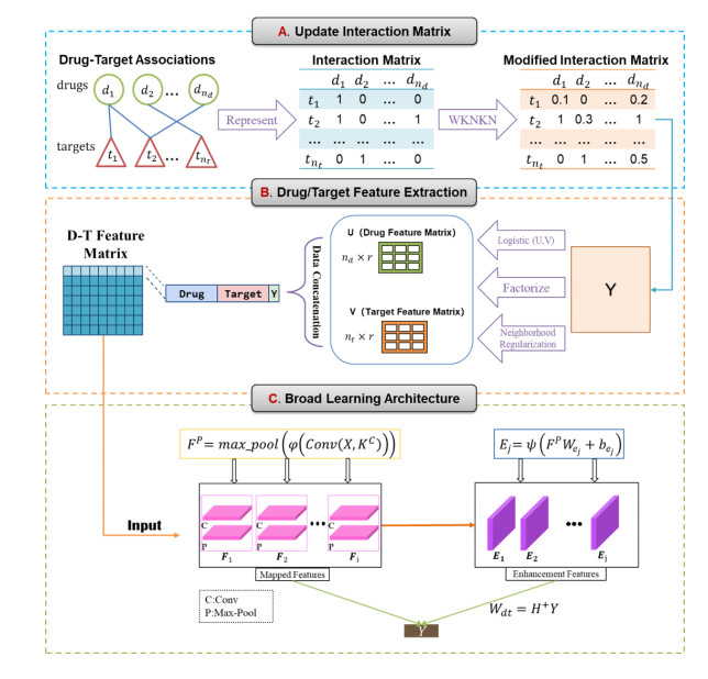
In the drug discovery process, time and costs are the most typical problems resulting from the experimental screening of drug-target interactions (DTIs). To address these limitations, many computational methods have been developed to achieve more accurate predictions. However, identifying DTIs mostly rely on separate learning tasks with drug and target features that neglect interaction representation between drugs and target. In addition, the lack of these relationships may lead to a greatly impaired performance on the prediction of DTIs. Aiming at capturing comprehensive drug-target representations and simplifying the network structure, we propose an integrative approach with a convolution broad learning system for the DTI prediction (ConvBLS-DTI) to reduce the impact of the data sparsity and incompleteness. First, given the lack of known interactions for the drug and target, the weighted K-nearest known neighbors (WKNKN) method was used as a preprocessing strategy for unknown drug-target pairs. Second, a neighborhood regularized logistic matrix factorization (NRLMF) was applied to extract features of updated drug-target interaction information, which focused more on the known interaction pair parties. Then, a broad learning network incorporating a convolutional neural network was established to predict DTIs, which can make classification more effective using a different perspective. Finally, based on the four benchmark datasets in three scenarios, the ConvBLS-DTI's overall performance out-performed some mainstream methods. The test results demonstrate that our model achieves improved prediction effect on the area under the receiver operating characteristic curve and the precision-recall curve.

| [1] |
X. Lin, S. Xu, X. Liu, X. Zhang, J. Hu, Detecting drug-target interactions with feature similarity fusion and molecular graphs, Biology (Basel), 11 (2022), 967. https://doi.org/10.3390/biology11070967 doi: 10.3390/biology11070967

|
| [2] |
N. R. C. Monteiro, B. Ribeiro, J. P. Arrais, Drug-target interaction prediction: End-to-end deep learning approach, IEEE/ACM Trans. Comput. Biol. Bioinf., 18 (2021), 2364–2374. https://doi.org/10.1109/TCBB.2020.2977335 doi: 10.1109/TCBB.2020.2977335
|
| [3] |
R. Chen, X. Liu, S. Jin, J. Lin, J. Liu, Machine learning for drug-target interaction prediction, Molecules, 23 (2018), 2208. https://doi.org/10.3390/molecules23092208 doi: 10.3390/molecules23092208
|
| [4] |
J. P. Hughes, S. Rees, S. B. Kalindjian, K. L. Philpott, Principles of early drug discovery, Br. J. Pharmacol., 162 (2011), 1239–1249. https://doi.org/10.1111/j.1476-5381.2010.01127.x doi: 10.1111/j.1476-5381.2010.01127.x
|
| [5] |
M. Rudrapal, D. Chetia, Virtual screening, molecular docking and QSAR studies in drug discovery and development programme, J. Drug Deliv. Sci. Ther., 10 (2020), 225–233. https://doi.org/10.22270/jddt.v10i4.4218 doi: 10.22270/jddt.v10i4.4218
|
| [6] |
Q. Ye, C. Y. Hsieh, Z. Yang, Y. Kang, J. Chen, D. Cao, et al., A unified drug-target interaction prediction framework based on knowledge graph and recommendation system, Nat. Commun., 12 (2021), 6775. https://doi.org/10.1038/s41467-021-27137-3 doi: 10.1038/s41467-021-27137-3
|
| [7] |
S. Luukkonen, H. W. van den Maagdenberg, M. T. M. Emmerich, G. J. P. van Westen, Artificial intelligence in multi-objective drug design, Curr. Opin. Struct. Biol., 79 (2023), 102537. https://doi.org/10.1016/j.sbi.2023.102537 doi: 10.1016/j.sbi.2023.102537
|
| [8] |
F. Li, Z. Zhang, J. Guan, S. Zhou, Effective drug-target interaction prediction with mutual interaction neural network, Bioinformatics, 38 (2022), 3582–3589. https://doi.org/10.1093/bioinformatics/btac377 doi: 10.1093/bioinformatics/btac377
|
| [9] |
M. Bagherian, E. Sabeti, K. Wang, M. A. Sartor, Z. Nikolovska-Coleska, K. Najarian, Machine learning approaches and databases for prediction of drug-target interaction: A survey paper, Brief Bioinf., 22 (2021), 247–269. https://doi.org/10.1093/bib/bbz157 doi: 10.1093/bib/bbz157
|
| [10] |
J. P. Mei, C. K. Kwoh, P. Yang, X. L. Li, J. Zheng, Drug-target interaction prediction by learning from local information and neighbors, Bioinformatics, 29 (2013), 238–245. https://doi.org/10.1093/bioinformatics/bts670 doi: 10.1093/bioinformatics/bts670
|
| [11] |
Y. Luo, X. Zhao, J. Zhou, J. Yang, Y. Zhang, W. Kuang, et al., A network integration approach for drug-target interaction prediction and computational drug repositioning from heterogeneous information, Nat. Commun., 8 (2017), 573. https://doi.org/10.1038/s41467-017-00680-8 doi: 10.1038/s41467-017-00680-8
|
| [12] |
A. Ezzat, P. Zhao, M. Wu, X. L. Li, C. K. Kwoh, Drug-target interaction prediction with graph regularized matrix factorization, IEEE/ACM Trans. Comput. Biol. Bioinform., 14 (2017), 646–656. https://doi.org/10.1109/TCBB.2016.2530062 doi: 10.1109/TCBB.2016.2530062
|
| [13] |
N. Zong, H. Kim, V. Ngo, O. Harismendy, Deep mining heterogeneous networks of biomedical linked data to predict novel drug-target associations, Bioinformatics, 33 (2017), 2337–2344. https://doi.org/10.1093/bioinformatics/btx160 doi: 10.1093/bioinformatics/btx160
|
| [14] |
M. Wen, Z. Zhang, S. Niu, H. Sha, R. Yang, Y. Yun, et al., Deep-learning-based drug-target interaction prediction, J. Proteome Res., 16 (2017), 1401–1409. https://doi.org/10.1021/acs.jproteome.6b00618 doi: 10.1021/acs.jproteome.6b00618
|
| [15] |
Y. B. Wang, Z. H. You, S. Yang, H. C. Yi, Z. H. Chen, K. Zheng, A deep learning-based method for drug-target interaction prediction based on long short-term memory neural network, BMC Med. Inf. Decis. Mak., 20 (2020), 49. https://doi.org/10.1186/s12911-020-1052-0 doi: 10.1186/s12911-020-1052-0
|
| [16] |
H. Öztürk, A. Özgür, E. Ozkirimli, DeepDTA: Deep drug-target binding affinity prediction, Bioinformatics, 34 (2018), i821–i829. https://doi.org/10.1093/bioinformatics/bty593 doi: 10.1093/bioinformatics/bty593
|
| [17] |
C. Chen, H. Shi, Z. Jiang, A. Salhi, R. Chen, X. Cui, et al., DNN-DTIs: Improved drug-target interactions prediction using XGBoost feature selection and deep neural network, Comput. Biol. Med., 136 (2021), 104676. https://doi.org/10.1016/j.compbiomed.2021.104676 doi: 10.1016/j.compbiomed.2021.104676
|
| [18] |
Q. Zhao, H. Zhao, K. Zheng, J. Wang, HyperAttentionDTI: improving drug-protein interaction prediction by sequence-based deep learning with attention mechanism, Bioinformatics, 38 (2022), 655–662. https://doi.org/10.1093/bioinformatics/btab715 doi: 10.1093/bioinformatics/btab715
|
| [19] |
S. Zheng, Y. Li, S. Chen, J. Xu, Y. Yang, Predicting drug–protein interaction using quasi-visual questionanswering system, Nat. Mach. Intell., 2 (2020), 134–140. https://doi.org/10.1038/s42256-020-0152-y doi: 10.1038/s42256-020-0152-y
|
| [20] |
T. Zhao, Y. Hu, L. R. Valsdottir, T. Zang, J. Peng, Identifying drug-target interactions based on graph convolutional network and deep neural network, Brief Bioinf., 22 (2021), 2141–2150. https://doi.org/10.1093/bib/bbaa044 doi: 10.1093/bib/bbaa044
|
| [21] |
M. Tsubaki, K. Tomii, J. Sese, Compound-protein interaction prediction with end-to-end learning of neural networks for graphs and sequences, Bioinformatics, 35 (2019), 309–318. https://doi.org/10.1093/bioinformatics/bty535 doi: 10.1093/bioinformatics/bty535
|
| [22] |
J. You, R. D. McLeod, P. Hu, Predicting drug-target interaction network using deep learning model, Comput. Biol. Chem., 80 (2019), 90–101. https://doi.org/10.1016/j.compbiolchem.2019.03.016 doi: 10.1016/j.compbiolchem.2019.03.016
|
| [23] |
M. A. Thafar, R. S. Olayan, S. Albaradei, V. B. Bajic, T. Gojobori, M. Essack, et al., DTi2Vec: Drug-target interaction prediction using network embedding and ensemble learning, J. Cheminf., 13 (2021), 71. https://doi.org/10.1186/s13321-021-00552-w doi: 10.1186/s13321-021-00552-w
|
| [24] |
K. Huang, C. Xiao, L. M. Glass, J. Sun, MolTrans: Molecular interaction transformer for drug-target interaction prediction, Bioinformatics, 37 (2021), 830–836. https://doi.org/10.1093/bioinformatics/btaa880 doi: 10.1093/bioinformatics/btaa880
|
| [25] |
J. Peng, J. Li, X. Shang, A learning-based method for drug-target interaction prediction based on feature representation learning and deep neural network, BMC Bioinf., 21 (2020), 394. https://doi.org/10.1186/s12859-020-03677-1 doi: 10.1186/s12859-020-03677-1
|
| [26] |
C. L. P. Chen, Z. L. Liu, Broad learning system: An effective and efficient incremental learning system without the need for deep architecture, EEE Trans. Neural Netw. Learn. Syst., 29 (2018), 10–24. https://doi.org/10.1109/Tnnls.2017.2716952 doi: 10.1109/Tnnls.2017.2716952
|
| [27] |
Y. H. Pao, Y. Takefuji, Functional-link net computing: theory, system architecture, and functionalities, Computer, 25 (1992), 76–79. https://doi.org/10.1109/2.144401 doi: 10.1109/2.144401
|
| [28] |
B. Igelnik, Y. H. Pao, Stochastic choice of basis functions in adaptive function approximation and the functional-link net, IEEE Trans. Neural Netw, 6 (1995), 1320–1329. https://doi.org/10.1109/72.471375 doi: 10.1109/72.471375
|
| [29] |
X. Gong, T. Zhang, C. L. P. Chen, Z. Liu, Research review for broad learning system: Algorithms, theory, and applications, IEEE Trans. Cybern., 52 (2022), 8922–8950. https://doi.org/10.1109/TCYB.2021.3061094 doi: 10.1109/TCYB.2021.3061094
|
| [30] |
X. N. Fan, S. W. Zhang, LPI-BLS: Predicting lncRNA–protein interactions with a broad learning system-based stacked ensemble classifier, Neurocomputing, 370 (2019), 88–93. https://doi.org/https://doi.org/10.1016/j.neucom.2019.08.084 doi: 10.1016/j.neucom.2019.08.084
|
| [31] |
K. Zheng, Z. H. You, L. Wang, Y. R. Li, H. J. Jiang, MISSIM: Improved miRNA-disease association prediction model based on chaos game representation and broad learning system, Intell. Comput. Methodol., 11645 (2019), 392–398. https://doi.org/10.1007/978-3-030-26766-7_36 doi: 10.1007/978-3-030-26766-7_36
|
| [32] |
Y. Liu, M. Wu, C. Miao, P. Zhao, X. L. Li, Neighborhood regularized logistic matrix factorization for drug-target interaction prediction, PLOS Comput. Biol., 12 (2016), e1004760. https://doi.org/10.1371/journal.pcbi.1004760 doi: 10.1371/journal.pcbi.1004760
|
| [33] |
A. E. Hoerl, R. W. Kennard, Ridge regression: Applications to nonorthogonal problems, Technometrics, 12 (2000), 55–67. https://doi.org/10.1080/00401706.1970.10488635 doi: 10.1080/00401706.1970.10488635
|
| [34] |
Y. Yamanishi, M. Araki, A. Gutteridge, W. Honda, M. Kanehisa, Prediction of drug-target interaction networks from the integration of chemical and genomic spaces, Bioinformatics, 24 (2008), 232–240. https://doi.org/10.1093/bioinformatics/btn162 doi: 10.1093/bioinformatics/btn162
|
| [35] |
B. Liu, D. Papadopoulos, F. D. Malliaros, G. Tsoumakas, A. N. Papadopoulos, Multiple similarity drug-target interaction prediction with random walks and matrix factorization, Brief Bioinf., 23 (2022), 1–10. https://doi.org/10.1093/bib/bbac353 doi: 10.1093/bib/bbac353
|
| [36] |
M. Kanehisa, M. Furumichi, M. Tanabe, Y. Sato, K. Morishima, KEGG: New perspectives on genomes, pathways, diseases and drugs, Nucleic Acids Res., 45 (2017), D353–D361. https://doi.org/10.1093/nar/gkw1092 doi: 10.1093/nar/gkw1092
|
| [37] |
D. S. Wishart, Y. D. Feunang, A. C. Guo, E. J. Lo, A. Marcu, J. R. Grant, et al., DrugBank 5.0: A major update to the drugbank database for 2018, Oxford Univ. Press, 46 (2018), D1074–D1082. https://doi.org/10.1093/nar/gkx1037 doi: 10.1093/nar/gkx1037
|
| [38] |
D. Mendez, A. Gaulton, A. P. Bento, J. Chambers, M. de Veij, E. Félix, et al., ChEMBL: Towards direct deposition of bioassay data, Nucleic Acids Res., 47 (2018), D930–D940. https://doi.org/10.1093/nar/gky1075 doi: 10.1093/nar/gky1075
|
| [39] |
Q. H. Kha, V. H. Le, T. N. K. Hung, N. T. K. Nguyen, N. Q. K. Le, Development and validation of an explainable machine learning-based prediction model for drug-food interactions from chemical structures, Sensors, 23 (2023), 3962. https://doi.org/10.3390/s23083962 doi: 10.3390/s23083962
|
| [40] |
N. Q. K. Le, T. T. D. Nguyen, Y. Y. M. Ou, Identifying the molecular functions of electron transport proteins using radial basis function networks and biochemical properties, J. Mol. Graphi. Model., 73 (2017), 166–178. https://doi.org/10.1016/j.jmgm.2017.01.003 doi: 10.1016/j.jmgm.2017.01.003
|
| [41] |
M. Schrynemackers, R. Küffner, P. Geurts, On protocols and measures for the validation of supervised methods for the inference of biological networks, Front. Gene., 4 (2013), 262. https://doi.org/10.3389/fgene.2013.00262 doi: 10.3389/fgene.2013.00262
|
| [42] |
B. Liu, K. Pliakos, C. Vens, G. Tsoumakas, Drug-target interaction prediction via an ensemble of weighted nearest neighbors with interaction recovery, Appl. Intell., 52 (2022), 3705–3727. https://doi.org/10.1007/s10489-021-02495-z doi: 10.1007/s10489-021-02495-z
|
| [43] |
M. A. Thafar, R. S. Olayan, S. Albaradei, V. B. Bajic, T. Gojobori, M. Essack, et al., DTi2Vec: Drug-target interaction prediction using network embedding and ensemble learning, J. Cheminf., 71 (2021), 1–18. https://doi.org/10.1186/S13321-021-00552-W doi: 10.1186/S13321-021-00552-W
|
| [44] |
J. Zhang, M. Xie, Graph regularized non-negative matrix factorization with prior knowledge consistency constraint for drug-target interactions prediction, BMC Bioinf., 23 (2022), 1–20. https://doi.org/10.1186/s12859-022-05119-6 doi: 10.1186/s12859-022-05119-6
|


Figures(6) / Tables(8)

Wanying Xu, Xixin Yang, Yuanlin Guan, Xiaoqing Cheng, Yu Wang. Integrative approach for predicting drug-target interactions via matrix factorization and broad learning systems[J]. Mathematical Biosciences and Engineering, 2024, 21(2): 2608-2625. doi: 10.3934/mbe.2024115


 DownLoad: