In the field of state-of-the-art object detection, the task of object localization is typically accomplished through a dedicated subnet that emphasizes bounding box regression. This subnet traditionally predicts the object's position by regressing the box's center position and scaling factors. Despite the widespread adoption of this approach, we have observed that the localization results often suffer from defects, leading to unsatisfactory detector performance. In this paper, we address the shortcomings of previous methods through theoretical analysis and experimental verification and present an innovative solution for precise object detection. Instead of solely focusing on the object's center and size, our approach enhances the accuracy of bounding box localization by refining the box edges based on the estimated distribution at the object's boundary. Experimental results demonstrate the potential and generalizability of our proposed method.
Citation: Peng Zhi, Haoran Zhou, Hang Huang, Rui Zhao, Rui Zhou, Qingguo Zhou. Boundary distribution estimation for precise object detection[J]. Electronic Research Archive, 2023, 31(8): 5025-5038. doi: 10.3934/era.2023257
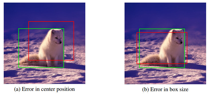
In the field of state-of-the-art object detection, the task of object localization is typically accomplished through a dedicated subnet that emphasizes bounding box regression. This subnet traditionally predicts the object's position by regressing the box's center position and scaling factors. Despite the widespread adoption of this approach, we have observed that the localization results often suffer from defects, leading to unsatisfactory detector performance. In this paper, we address the shortcomings of previous methods through theoretical analysis and experimental verification and present an innovative solution for precise object detection. Instead of solely focusing on the object's center and size, our approach enhances the accuracy of bounding box localization by refining the box edges based on the estimated distribution at the object's boundary. Experimental results demonstrate the potential and generalizability of our proposed method.

| [1] |
R. Kaur, S. Singh, A comprehensive review of object detection with deep learning, Digital Signal Process., 132 (2023), 103812. https://doi.org/10.1016/j.dsp.2022.103812 doi: 10.1016/j.dsp.2022.103812

|
| [2] |
P. Jiang, D. Ergu, F. Liu, Y. Cai, B. Ma, A Review of Yolo algorithm developments, Proc. Comput. Sci., 199 (2022), 1066–1073. https://doi.org/10.1016/j.procs.2022.01.135 doi: 10.1016/j.procs.2022.01.135
|
| [3] |
W. Liu, G. Wu, F. Ren, X. Kang, DFF-ResNet: An insect pest recognition model based on residual networks, Big Data Min. Anal., 3 (2020), 300–310. https://doi.org/10.26599/BDMA.2020.9020021 doi: 10.26599/BDMA.2020.9020021
|
| [4] |
A. Mughees, L. Tao, Multiple deep-belief-network-based spectral-spatial classification of hyperspectral images, Tsinghua Sci. Technol., 24 (2019), 183–194. https://doi.org/10.26599/TST.2018.9010043 doi: 10.26599/TST.2018.9010043
|
| [5] | T. Y. Lin, M. Maire, S. Belongie, J. Hays, P. Perona, D. Ramanan, et al., Microsoft COCO: Common objects in context, in European Conference on Computer Vision, (2014), 740–755. https://doi.org/10.1007/978-3-319-10602-1_48 |
| [6] |
O. Russakovsky, J. Deng, H. Su, J. Krause, S. Satheesh, S. Ma, et al., ImageNet large scale visual recognition challenge, Int. J. Comput. Vis., 115 (2015), 211–252. https://doi.org/10.1007/s11263-015-0816-y doi: 10.1007/s11263-015-0816-y
|
| [7] |
Y. Fan, D. Ni, H. Ma, HyperDB: a hyperspectral land class database designed for an image processing system, Tsinghua Sci. Technol., 22 (2017), 112–118. https://doi.org/10.1109/TST.2017.7830901 doi: 10.1109/TST.2017.7830901
|
| [8] |
M. Everingham, S. M. A. Eslami, L. Van Gool, C. K. I. Williams, J. Winn, A. Zisserman, The PASCAL visual object classes challenge: A retrospective, Int. J. Comput. Vis., 111 (2015), 98–136. https://doi.org/10.1007/s11263-014-0733-5 doi: 10.1007/s11263-014-0733-5
|
| [9] |
S. Ren, K. He, R. Girshick, J. Sun, Faster R-CNN: Towards real-time object detection with region proposal networks, IEEE Trans. Pattern Anal. Mach. Intell., 39 (2017), 1137–1149. https://doi.org/10.1109/TPAMI.2016.2577031 doi: 10.1109/TPAMI.2016.2577031
|
| [10] | T. Y. Lin, P. Goyal, R. Girshick, K. He, P. Dollár, Focal loss for dense object detection, in 2017 IEEE International Conference on Computer Vision (ICCV), (2017), 2999–3007. https://doi.org/10.1109/ICCV.2017.324 |
| [11] | X. Zhou, D. Wang, P. Krähenbühl, Objects as points, preprint, arXiv: 1904.07850. |
| [12] |
K. He, G. Gkioxari, P. Dollár, R. Girshick, Mask R-CNN, IEEE Trans. Pattern Anal. Mach. Intell., 42 (2020), 386–397. https://doi.org/10.1109/TPAMI.2018.2844175 doi: 10.1109/TPAMI.2018.2844175
|
| [13] | M. Chen, F. Bai, Z. Gerile, Special object detection based on Mask RCNN, in 2021 17th International Conference on Computational Intelligence and Security (CIS), (2021), 128–132. https://doi.org/10.1109/CIS54983.2021.00035 |
| [14] |
Z. Ou, Z. Wang, F. Xiao, B. Xiong, H. Zhang, M. Song, et al., AD-RCNN: Adaptive dynamic neural network for small object detection, IEEE Int. Things J., 10 (2023), 4226–4238. https://doi.org/10.1109/JIOT.2022.3215469 doi: 10.1109/JIOT.2022.3215469
|
| [15] |
L. Yang, Y. Xu, S. Wang, C. Yang, Z. Zhang, B. Li, et al., PDNet: Toward better one-stage object detection with prediction decoupling, IEEE Trans. Image Process., 31 (2022), 5121–5133. https://doi.org/10.1109/TIP.2022.3193223 doi: 10.1109/TIP.2022.3193223
|
| [16] | J. Redmon, S. Divvala, R. Girshick, A. Farhadi, You only look once: Unified, real-time object detection, in 2016 IEEE Conference on Computer Vision and Pattern Recognition (CVPR), (2016), 770–778. https://doi.ieeecomputersociety.org/10.1109/CVPR.2016.91 |
| [17] | W. Liu, D. Anguelov, D. Erhan, C. Szegedy, S. Reed, C. Y. Fu, et al., SSD: Single shot multiBox detector, in European Conference on Computer Vision, (2016), 21–37. https://doi.org/10.1007/978-3-319-46448-0_2 |
| [18] | J. Redmon, A. Farhadi, YOLOv3: An incremental improvement, preprint, arXiv: 1804.02767. |
| [19] |
G. Wang, J. Wu, B. Tian, S. Teng, L. Chen, D. Cao, et al., CenterNet3D: An anchor free object detector for point cloud, IEEE Trans. Intell. Transp. Syst., 23 (2022), 12953–12965. https://doi.org/10.1109/TITS.2021.3118698 doi: 10.1109/TITS.2021.3118698
|
| [20] | Z. Tian, C. Shen, H. Chen, T. He, FCOS: Fully convolutional one-stage object detection, in 2019 IEEE/CVF International Conference on Computer Vision (ICCV), (2019), 9626–9635. https://doi.ieeecomputersociety.org/10.1109/ICCV.2019.00972 |
| [21] |
H. Law, J. Deng, CornerNet: Detecting objects as paired keypoints, Int. J. Comput. Vis., 128 (2020), 642–656. https://doi.org/10.1007/s11263-019-01204-1 doi: 10.1007/s11263-019-01204-1
|
| [22] |
J. Canny, A computational approach to edge detection, IEEE Trans. Pattern Anal. Mach. Intell., 8 (1986), 679–698. https://doi.org/10.1109/TPAMI.1986.4767851 doi: 10.1109/TPAMI.1986.4767851
|
| [23] |
D. Marr, E. Hildreth, Theory of edge detection, Proc. R. Soc. Lond. B, 207 (1980), 187–217. https://doi.org/10.1098/rspb.1980.0020 doi: 10.1098/rspb.1980.0020
|
| [24] |
J. Kittler, On the accuracy of the Sobel edge detector, Image Vis. Comput., 1 (1983), 37–42. https://doi.org/10.1016/0262-8856(83)90006-9 doi: 10.1016/0262-8856(83)90006-9
|
| [25] |
D. R. Martin, C. C. Fowlkes, J. Malik, Learning to detect natural image boundaries using local brightness, color, and texture cues, IEEE Trans. Pattern Anal. Mach. Intell., 26 (2004), 530–549. https://doi.org/10.1109/TPAMI.2004.1273918 doi: 10.1109/TPAMI.2004.1273918
|
| [26] |
P. Arbeláez, M. Maire, C. Fowlkes, J. Malik, Contour detection and hierarchical image segmentation, IEEE Trans. Pattern Anal. Mach. Intell., 33 (2011), 898–916. https://doi.org/10.1109/TPAMI.2010.161 doi: 10.1109/TPAMI.2010.161
|
| [27] | J. J. Lim, C. L. Zitnick, P. Dollár, Sketch tokens: A learned mid-level representation for contour and object detection, in 2013 IEEE Conference on Computer Vision and Pattern Recognitionn, (2013), 3158–3165. https://doi.org/10.1109/CVPR.2013.406 |
| [28] | P. Dollár, C. L. Zitnick, Structured forests for fast edge detection, in 2013 IEEE International Conference on Computer Vision, (2013), 1841–1848. https://doi.org/10.1109/ICCV.2013.231 |
| [29] | S. Xie, Z. Tu, Holistically-nested edge detection, in 2015 IEEE International Conference on Computer Vision (ICCV), (2015), 1395–1403. https://doi.org/10.1109/ICCV.2015.164 |
| [30] | G. Bertasius, J. Shi, L. Torresani, DeepEdge: A multi-scale bifurcated deep network for top-down contour detection, in 2015 IEEE Conference on Computer Vision and Pattern Recognition (CVPR), (2015), 4380–4389. https://doi.org/10.1109/CVPR.2015.7299067 |
| [31] | W. Shen, X. Wang, Y. Wang, X. Bai, Z. Zhang, DeepContour: A deep convolutional feature learned by positive-sharing loss for contour detection, in 2015 IEEE Conference on Computer Vision and Pattern Recognition (CVPR), (2015), 3982–3991. https://doi.org/10.1109/CVPR.2015.7299024 |
| [32] | Z. Huang, L. Huang, Y. Gong, C. Huang, X. Wang, Mask scoring R-CNN, in 2019 IEEE/CVF Conference on Computer Vision and Pattern Recognition (CVPR), (2019), 6402–6411. https://doi.org/10.1109/CVPR.2019.00657 |
| [33] | K. Chen, J. Pang, J. Wang, Y. Xiong, X. Li, S. Sun, et al., Hybrid task cascade for instance segmentation, in 2019 IEEE/CVF Conference on Computer Vision and Pattern Recognition (CVPR), (2019), 4974–4983. https://doi.org/10.1109/CVPR.2019.00511 |
| [34] | C. L. Zitnick, P. Dollár, Edge boxes: Locating object proposals from edges, in European Conference on Computer Vision, (2014), 391–405. https://doi.org/10.1007/978-3-319-10602-1_26 |
| [35] | J. Dai, H. Qi, Y. Xiong, Y. Li, G. Zhang, H. Hu, et al., Deformable convolutional networks, in 2017 IEEE International Conference on Computer Vision (ICCV), (2017), 764–773. https://doi.org/10.1109/ICCV.2017.89 |
| [36] | Y. Kim, T. Kim, B. N. Kang, J. Kim, D. Kim, BAN: Focusing on boundary context for object detection, in Asian Conference on Computer Vision, (2018), 555–570. https://doi.org/10.1007/978-3-030-20876-9_35 |
| [37] | J. Wang, W. Zhang, Y. Cao, K. Chen, J. Pang, T. Gong, et al., Side-aware boundary localization for more precise object detection, in European Conference on Computer Vision, (2020), 403–419. https://doi.org/10.1007/978-3-030-58548-8_24 |
| [38] | C. Y. Fu, W. Liu, A. Ranga, A. Tyagi, A. C. Berg, DSSD: Deconvolutional single shot detector, preprint, arXiv: 1701.06659. |
| [39] | R. Araki, T. Onishi, T. Hirakawa, T. Yamashita, H. Fujiyoshi, MT-DSSD: Deconvolutional single shot detector using multi task learning for object detection, segmentation, and grasping detection, in 2020 IEEE International Conference on Robotics and Automation (ICRA), (2020), 10487–10493. https://doi.org/10.1109/ICRA40945.2020.9197251 |
| [40] | C. Y. Fu, M. Shvets, A. C. Berg, RetinaMask: Learning to predict masks improves state-of-the-art single-shot detection for free, preprint, arXiv: 1901.03353. |
| [41] | R. K. Meleppat, M. V. Matham, L. K. Seah, Optical frequency domain imaging with a rapidly swept laser in the 1300nm bio-imaging window, in International Conference on Optical and Photonic Engineering, (2015), 721–729. https://doi.org/10.1117/12.2190530 |
| [42] |
R. K. Meleppat, C. R. Fortenbach, Y. Jian, E. S. Martinez, K. Wagner, B. S. Modjtahedi, et al., In Vivo Imaging of Retinal and Choroidal Morphology and Vascular Plexuses of Vertebrates Using Swept-Source Optical Coherence Tomography, Transl. Vis. Sci. Technol., 11 (2022), 11. https://doi.org/10.1167/tvst.11.8.11 doi: 10.1167/tvst.11.8.11
|
| [43] | H. Huang, Research on Object Detection Based on Improved MASK R-CNN, Master's degree, Lanzhou University in Lanzhou, 2021. https://doi.org/10.27204/d.cnki.glzhu.2021.001818 |


Figures(6) / Tables(4)
Peng Zhi, Haoran Zhou, Hang Huang, Rui Zhao, Rui Zhou, Qingguo Zhou. Boundary distribution estimation for precise object detection[J]. Electronic Research Archive, 2023, 31(8): 5025-5038. doi: 10.3934/era.2023257


 DownLoad: