Threshold control strategy for a Filippov model with group defense of pests and a constant-rate release of natural enemies

Baolin Kang; Xiang Hou; Bing Liu; Baolin Kang; Xiang Hou; Bing Liu

doi:10.3934/mbe.2023537

Mathematical Biosciences and Engineering

2023, Volume 20, Issue 7: 12076-12092. doi: 10.3934/mbe.2023537

Previous Article Next Article

Research article Special Issues

Threshold control strategy for a Filippov model with group defense of pests and a constant-rate release of natural enemies

1.
College of Mathematics and Information Science, Anshan Normal University, Anshan 114007, China
2.
Research Center for Theoretical Ecology, School of Geography and Environment, Jiangxi Normal University, Nanchang 330022, China

Academic Editor: Yan Liu

Received: 29 January 2023 Revised: 27 March 2023 Accepted: 17 April 2023 Published: 15 May 2023

In this paper, we establish an integrated pest management Filippov model with group defense of pests and a constant rate release of natural enemies. First, the dynamics of the subsystems in the Filippov system are analyzed. Second, the dynamics of the sliding mode system and the types of equilibria of the Filippov system are discussed. Then the complex dynamics of the Filippov system are investigated by using numerical analysis when there is a globally asymptotically stable limit cycle and a globally asymptotically stable equilibrium in two subsystems, respectively. Furthermore, we analyze the existence region of a sliding mode and pseudo equilibrium, as well as the complex dynamics of the Filippov system, such as boundary equilibrium bifurcation, the grazing bifurcation, the buckling bifurcation and the crossing bifurcation. These complex sliding bifurcations reveal that the selection of key parameters can control the population density no more than the economic threshold, so as to prevent the outbreak of pests.

Keywords:

Citation: Baolin Kang, Xiang Hou, Bing Liu. Threshold control strategy for a Filippov model with group defense of pests and a constant-rate release of natural enemies[J]. Mathematical Biosciences and Engineering, 2023, 20(7): 12076-12092. doi: 10.3934/mbe.2023537

Related Papers:

[1]	Menita Carozza, Luca Esposito, Raffaella Giova, Francesco Leonetti . Polyconvex functionals and maximum principle. Mathematics in Engineering, 2023, 5(4): 1-10. doi: 10.3934/mine.2023077
[2]	Federico Cluni, Vittorio Gusella, Dimitri Mugnai, Edoardo Proietti Lippi, Patrizia Pucci . A mixed operator approach to peridynamics. Mathematics in Engineering, 2023, 5(5): 1-22. doi: 10.3934/mine.2023082
[3]	Italo Capuzzo Dolcetta . The weak maximum principle for degenerate elliptic equations: unbounded domains and systems. Mathematics in Engineering, 2020, 2(4): 772-786. doi: 10.3934/mine.2020036
[4]	Isabeau Birindelli, Kevin R. Payne . Principal eigenvalues for k-Hessian operators by maximum principle methods. Mathematics in Engineering, 2021, 3(3): 1-37. doi: 10.3934/mine.2021021
[5]	Francesco Cordoni, Luca Di Persio . A maximum principle for a stochastic control problem with multiple random terminal times. Mathematics in Engineering, 2020, 2(3): 557-583. doi: 10.3934/mine.2020025
[6]	Lucio Boccardo . Weak maximum principle for Dirichlet problems with convection or drift terms. Mathematics in Engineering, 2021, 3(3): 1-9. doi: 10.3934/mine.2021026
[7]	Qiang Du, Tadele Mengesha, Xiaochuan Tian . $L^{p}$ compactness criteria with an application to variational convergence of some nonlocal energy functionals. Mathematics in Engineering, 2023, 5(6): 1-31. doi: 10.3934/mine.2023097
[8]	Michael Herrmann, Karsten Matthies . Solitary waves in atomic chains and peridynamical media. Mathematics in Engineering, 2019, 1(2): 281-308. doi: 10.3934/mine.2019.2.281
[9]	Marco Cirant, Kevin R. Payne . Comparison principles for viscosity solutions of elliptic branches of fully nonlinear equations independent of the gradient. Mathematics in Engineering, 2021, 3(4): 1-45. doi: 10.3934/mine.2021030
[10]	Patrizia Pucci, Letizia Temperini . On the concentration–compactness principle for Folland–Stein spaces and for fractional horizontal Sobolev spaces. Mathematics in Engineering, 2023, 5(1): 1-21. doi: 10.3934/mine.2023007

Abstract

1. Introduction

Every woman is susceptible to breast cancer. Breast cancer is the second most lethal cancer after lung cancer, according to data from the World Health Organization (WHO) from 2004. The tumor, lymph node, metastasis (TNM) system establishes the malignancy phase [1]. The tumor size (T), the number of lymph nodes (N), and the spread (Metastasis) to other sites (M) are used by the TNM system to determine the degree of malignancy. If the cancer is identified in its early stages, the recovery from breast disease is not at all difficult. There is less chance of recovery as the stage increases. There are several different types of cancer medications, including chemotherapy, radiotherapy, hormone therapy, focused therapy and other claimed medical treatments. Cancer treatment kills cancer cells, prevents cancer cells from becoming cancer cells, or prevents cancer cells from receiving signals for cell proliferation. In this paper, we create a numerical model to analyze the effects of chemotherapy on the hearts of patients and the stages of breast cancer [2].

Models of heart failure based on the cardiotoxicity of anticancer medications are discussed in [1] and [3], dissecting cancer through mathematics: from the cell to the animal model in [4], a mathematical model analysis of breast cancer stages with heart side effects in chemotherapy patients in [5], optimal control and solution of the cellular DNA cancer model in [6], optimal control is used to study the dynamical behaviors of fractional financial awareness models in [7]. In [8], a Caputo-Fabrizio derivative is used to solve fractional glioblastoma multiforme. In [9] studies numerical, approximate solutions and optimal control of Lassa Hemorrhagic Fever in pregnant women. In [10] studies on a general formulation for numerical optimization of control problems and [11] the formulation of Euler-Lagrange equations for fractional variational problems. A formulation and numerical scheme for fractional optimal control problems are presented in [12]. In [13], fractional optimal control problems with multiple states and control variables are considered. A numerical method for solving the nonlinear equations of Emden-Fowler models is described in [14] and a numerical approach is used in optimal control [15] for a nonlinear mathematical model of the tumor under immune suppression. [16] studies optimal control for a fractional tuberculosis infection model taking diabetes and resistant strains into account and a numerical approach to fractional optimal control in the transmission dynamics of the West Nile model with state and control time delays is presented in [17]. [18] describes numerical treatments of West Nile virus transmission dynamics and optimal control. Studies on the dynamics of a fractional mathematical model of cancer tumor disease are presented in [19]. Approximate numerical methods for mathematical and physical studies for COVID-19 models are discussed in [20]. The 3-dimensional multispecies nonlinear tumor growth-I: model and numerical approach is studied in [21]. Studies [22] used symmetry approaches on a mathematical model of a brain tumor. The fractional-order susceptible-infected-susceptible (SIS) epidemic model with variable population size is described in [23]. An equation of fractional diffusion is used to simulate a cancer tumor in investigations [24]. The optimal control and spectral colocation method for solving smoking models are described in [25]. In [26], the authors present a numerical solution and dynamical behaviors for solving a fractional nonlinear rubella disease model. Dynamical behaviors of a nonlinear coronavirus (COVID-19) model with numerical studies are described in [27]. The fractional mathematical model for the concentration of tumor cells for a constant death rate has analytical solutions in [28] research. The fractional-order mathematical model that underlies immune chemotherapeutic therapy for breast cancer was numerically investigated in studies [29] employing neural networks. A non-local tumor growth model has solutions and numerical approximations in works by [30]. The numerical solutions for a tumor cell invasion and migration model in [31] studies. Computational simulations for solving nonlinear composite oscillation fractional are described in [32]. For the chaotic-cancer-model, investigations [33] enhanced the numerical solutions. [34] studies general fractional financial models of awareness using the Caputo Fabrizio derivative. [35] studies algorithms for fractional calculus using a variety of numerical methods. [36] studies finite-time event-triggered adaptive neural control for fractional-order nonlinear systems. Event-triggered adaptive neural control of fractional-order nonlinear systems with full-state constraints is described in [37]. [38] studies adaptive asymptotic tracking of nonlinear systems with unknown virtual control coefficients using the Barrier Lyapunov function. A fractional mathematical model of the breast cancer competition model is described in [39].

We provide a brand-new fractional numerical model of the stages of bosom disease with cardiac findings that demonstrate the existence of a stable arrangement in the partial model. Additionally explored are the model's ideal control and the mathematical procedure for simulating the control problem. With the help of mathematical games, we were able to attain the investigation's results. Similar to this, when various starting conditions are applied, the mathematics have a conclusion, which is supposedly a balance point that is constantly steady without conditions.

The paper is organized as follows: A predictor-corrector approach, marking, and preliminary work have been represented in Section 2. In Section 2, we also used a signal flow diagram to illustrate the cancer model. In Section 3, we talked about the uniformly stable solution after control and the optimal control (OC) for the fractional cancer model. In Section 4, we have resolved the nonlinear fractional cancer model using a predictor-corrector approach. The cancer model has been numerically simulated in Section 5. In Section 6, conclusions have been discussed. We describe the upcoming work in Section 7.

2. Methods

2.1. Preparations and marking

The following are some essential advantages and benefits of the concept of fractional calculus that will be helpful in this paper:

Definition 2.1. In Caputo's sense, the derivative fractional (Δ^r) is [6],[26],[32],[35]:

$Δ^{r} A (t) = \frac{1}{Γ (n - r)} {\int_{0}^{t} (t - η)}^{n - r - 1} A^{(n)} (η) d η, for n - 1 < r \leq n, n \in Ν .$ (2.1)

Definition 2.2. [35] can be used for r > 0 to introduce the order derivative fractional Caputo r overall space, as Δ^r intended:

${}^{c}Δ_{+}^{r} A (t) = \frac{1}{Γ (n - r)} \int_{- \infty}^{t} {(t - η)}^{n - r - 1} Δ^{n} f (η) d η .$ (2.2)

2.2. Predictor-corrector method algorithm

The following system of variable fractional order differential equations will be solved using the predictor-corrector method algorithm [34],[35], which we shall present.

$\begin{array}{l} Δ^{r_{1}} x (t) = A_{1} (x, y, z), \\ Δ^{r_{2}} y (t) = A_{2} (x, y, z), 0 \leq t \leq T . \\ Δ^{r_{3}} z (t) = A_{3} (x, y, z), \end{array}$

with 0 < r_j ≤ 1 (j = 1,2,3) and initial condition (x₀, y₀, z₀).

(1) Determine these predicted values:

$\begin{array}{l} x_{m + 1}^{q} = x_{0} + \sum_{j = 0}^{m} \frac{β_{1, j, m + 1}}{Γ (r_{1} (t_{m + 1}))} A_{1} (x_{j}, y_{j}, z_{j}), \\ y_{m + 1}^{q} = y_{0} + \sum_{j = 0}^{m} \frac{β_{2, j, m + 1}}{Γ (r_{2} (t_{m + 1}))} A_{2} (x_{j}, y_{j}, z_{j}), \\ z_{m + 1}^{q} = z_{0} + \sum_{j = 0}^{m} \frac{β_{3, j, m + 1}}{Γ (r_{3} (t_{m + 1}))} A_{3} (x_{j}, y_{j}, z_{j}), \end{array}$

where

$β_{i, j, m + 1} = \frac{k^{r_{i}}}{r_{i}} [{(m - j + 1)}^{r_{i}} - {(m - j)}^{r_{i}}] . k = \frac{T}{M}, T_{m} = m k .$

(2) Perform the following analysis on the corrected values:

$\begin{array}{l} x_{m + 1} = x_{0} + \frac{k^{r_{1}}}{Γ (r_{1} (t_{m + 1}) + 2)} + A_{1} (x_{m + 1}^{q}, y_{m + 1}^{q}, z_{m + 1}^{q}) + \sum_{j = 0}^{m} \frac{k^{r_{1}} β_{1, j, m + 1} γ_{1, j, m + 1}}{Γ (r_{1} (t_{m + 1}) + 2)} A_{1} (x_{j}, y_{j}, z_{j}), \\ y_{m + 1}^{q} = y_{0} + \frac{k^{r_{2}}}{Γ (r_{2} (t_{m + 1}) + 2)} + A_{2} (x_{m + 1}^{q}, y_{m + 1}^{q}, z_{m + 1}^{q}) + \sum_{j = 0}^{m} \frac{k^{r_{1}} β_{2, j, m + 1} γ_{2, j, m + 1}}{Γ (r_{2} (t_{m + 1}) + 2)} A_{2} (x_{j}, y_{j}, z_{j}), where \\ z_{m + 1}^{q} = z_{0} + \frac{k^{r_{3}}}{Γ (r_{3} (t_{m + 1}) + 2)} + A_{3} (x_{m + 1}^{q}, y_{m + 1}^{q}, z_{m + 1}^{q}) + \sum_{j = 0}^{m} \frac{k^{r_{3}} β_{3, j, m + 1} γ_{3, j, m + 1}}{Γ (r_{3} (t_{m + 1}) + 2)} A_{3} (x_{j}, y_{j}, z_{j}), \end{array}$

$γ_{1, j, m + 1} = {\begin{cases} m^{r_{i} + 1} - (m - r_{i}) {(m + 1)}^{r_{i}}, j = 0, \\ {(m - j - 2)}^{r_{i} + 1} + {(m - j)}^{r_{i} + 1} - 2 {(m - j + 1)}^{r_{i}}, 1 \leq j \leq m, \\ 1, j = m + 1. \end{cases}$

See [40],[41] for more information on the method.

2.3. Our proposed model

The following innovative mathematical fractional of cancer mamma stages with cardiac side effects is researched in this piece for its approximative analytical solutions at r. The analytical approximate solution of the fractional order cancer model is the subject of recent research [5]:

$[\begin{matrix} Δ^{r} A \\ Δ^{r} B \\ Δ^{r} C \\ Δ^{r} D \\ Δ^{r} E \end{matrix}] = [\begin{matrix} θ_{1} \\ θ_{2} \\ θ_{3} \\ 0 \\ 0 \end{matrix}] + [\begin{matrix} - (µ_{A D} + µ_{A B}) & 0 & 0 & 0 & 0 \\ µ_{A B} & - (µ_{B D} + µ_{B C} + µ_{B C} + γ_{2}) & 0 & µ_{B D} & 0 \\ 0 & µ_{B C} & - (µ_{C D} + µ_{C E} + γ_{3}) & µ_{D C} & 0 \\ µ_{A D} & µ_{B D} & µ_{C D} & - (µ_{D B} + µ_{D C} + µ_{D E}) & 0 \\ 0 & µ_{B E} & µ_{C E} & µ_{D E} & - γ_{1} \end{matrix}] [\begin{matrix} A \\ B \\ C \\ D \\ E \end{matrix}],$ (2.3)

with initial conditions A(0) = A₀, B(0) = B₀, C(0) = C₀, D(0) = D₀ and E(0) = E₀.

Five compartments representing different subpopulations of breast cancer patients were used to build the model. Variables A, B, C, D and E each represent a certain subpopulation. Patients with ductal carcinoma in situ, stages 1, 2A and 2B are represented by sub-population A. Cancer patients in stages 3A and 3B are represented by subpopulation B. Patients with stage 4 cancer make up subpopulation C. Cancer patients in subpopulation D who are free of the disease following chemotherapy are represented. Cancer cannot be observed in an environment free of sickness. Cardiotoxic cancer patients are expressed in sub-population E. In Figure 1, the sign stream diagram is displayed. A system of differential equations is used to express the rate of change for each subpopulation (1). Be aware of the set defined by $ψ = {(A, B, C, D, E) | A > 0, B > 0, C > 0, D > 0, E > 0} .$ It's important to notice that all of the parameters shown in Table 1 are taken to have positive values.

Figure 1: The signal flow diagram is a tool that may illustrate the relationships between the states of the system and give us access to graph-theoretic tools for finding novel system characteristics.

Figure 1. Graph of a signal, see [24],[26],[29],[30].

DownLoad: Full-Size Img PowerPoint

Table 1. The physical significance and description of each parameter.

Parameter	Description
θ₁ = 5	Number of patients examined to be in stages 1 and 2 of cancer
θ₂ = 20	The number of patients undergoing treatment for stage 3 cancer
θ₃ = 11	The number of patients examined to endure malignant growth in phase 4
µ_AB = 0.56	Rate increased from phase 1 or 2 to stage 3 (reformist illness)
µ_AD = 0.63	Pace of phase 1 or 2 patients who experience a total reaction
µ_BD = 0.35	The rate at which phase 3 sick people experience a total reaction
µ_BC = 0.62	Expanded average from phase 3 to phase 4 (reformist illness)
µ_BE = 0.3	Pace of phase 3 malignant growth chemotherapy in sick patients who experiment with cardiotoxic treatment
µ_CD = 0.42	Pace of Phase 4 patients undergoing total reaction
µ_CE = 0.3	The rate of phase 4 malignant growth chemotherapy in sick patients undergoing cardiotoxic treatment
µ_DB = 0.36	The rate of illness releases ill people who fall back to position 3
µ_DC = 0.42	The tempo of illness releases stickers that revert to arrangement 4
µ_DE = 0.3	Ailment release rate of sick people who experiment cardiotoxic treatment
γ₁ = 0.4	Cardiotoxic patients are dying at a faster rate
γ₂ = 0.5	Patients with stage 3 malignant growth are dying at a faster rate
γ₃ = 0.8	Patients with stage 4 malignant growth are dying at a faster rate

| Show Table

DownLoad: CSV

3. Numerical modeling

3.1. Optimal control for the fractional cancer model

This section explains the ideal control for the fractional cancer system.

$\begin{array}{l} Δ^{r} A = θ_{1} - µ_{A D} A - µ_{A B} A, \\ Δ^{r} B = θ_{2} + µ_{A B} A + µ_{D B} D - µ_{B D} B - µ_{B C} B - µ_{B E} B - γ_{2} B, \\ Δ^{r} C = θ_{3} + µ_{B C} B + µ_{D C} D - µ_{C D} C - µ_{C E} C - γ_{3} C, \\ Δ^{r} D = µ_{A D} A + µ_{B D} B + µ_{C D} C - µ_{D B} D - µ_{D C} D - µ_{D E} D, \\ Δ^{r} E = µ_{D E} D + µ_{C E} C + µ_{B E} B - γ_{1} E . \end{array}$ (3.1.1)

The equations (3.1.1) in R₅, generated from references [11]–[15],[18]–[21],[29], will be explained as follows: $\forall t \in [0, T_{f}] = [0, 1]$ , $Ω = {(µ_{C D}, µ_{B E}) \in (L^{\infty} \times L^{\infty}) | 0 \leq µ_{C D}, µ_{B E} \leq 1}$ ,

where T_f is time final, µ_CD(.) is the typical value of phase 4 patients testing a complete echo and µ_BE(.) is the average number of cancer patients receiving phase 3 chemotherapy who test for cardiotoxicity. µ_CD(.) and µ_BE(.) are the mechanisms for control. The standard is the space function L^∞ ${∥ t ∥}_{\infty} = \max_{j} | t_{j} |$ .

The functional goal was described as follows:

$J = \int_{0}^{T_{f}} [b_{1} A + b_{2} µ_{_{C D}}^{2} + b_{3} µ_{_{B E}}^{2}] d t,$ (3.1.2)

where b₁, b₂ and b₃ reflect the average of phase 3 cancer chemotherapy patients who experience cardiotoxicity and the measure of stage 4 patients who experiment with a full echo, respectively.

There are defined minimize functions

$J = \int_{0}^{T_{f}} ϕ d t,$ (3.1.3)

where $ϕ = [a_{1} A (t) + a_{2} µ_{_{C D}}^{2} (t) + a_{3} µ_{_{B E}}^{2} (t)],$

bound by the constraint

$Δ^{r} A = ϵ_{1}, Δ^{r} B = ϵ_{2}, Δ^{r} C = ϵ_{3}, Δ^{r} D = ϵ_{4}, Δ^{r} E = ϵ_{5},$ (3.1.4)

where $ϵ_{j} = ϵ (A, B, C, D, E, µ_{C D}, µ_{B E}, t), j = 1, 2, 3, 4, 5,$

met the initial cases' requirements:

$A (0) = A_{1}, B (0) = B_{1}, C (0) = C_{1}, D (0) = D_{1}, E (0) = E_{1} .$ (3.1.5)

For the objective of the fractional optimal control problem (FOCP), see [26]–[29]:

$J^{*} = \int_{0}^{T_{f}} [H - \sum_{i = 1}^{5} λ_{i} ϵ_{i}] d t .$ (3.1.6)

The control equation (3.1.1) and objective Hamiltonian (3.1.6) are shown be pursuing the following goals:

$H = ϕ + \sum_{i = 1}^{5} λ_{i} ϵ_{i},$ (3.1.7)

Therefore

$\begin{array}{l} H = a_{1} A + a_{2} µ_{_{C D}}^{2} + a_{3} µ_{_{B E}}^{2} + λ_{1} [θ_{1} - µ_{A D} A - µ_{A B} A] \\ + λ_{2} [θ_{2} + µ_{A B} A + µ_{D B} D - µ_{B D} B - µ_{B C} B - µ_{B E} B - γ_{2} B] \\ + λ_{3} [θ_{3} + µ_{B C} B + µ_{D C} D - µ_{C D} C - µ_{C E} C - γ_{3} C] \\ + λ_{4} [µ_{A D} A + µ_{B D} B + µ_{C D} C - µ_{D B} D - µ_{D C} D - µ_{D E} D] \\ + λ_{5} [µ_{D E} D + µ_{C E} C + µ_{B E} B - γ_{1} E] . \end{array}$ (3.1.8)

In [26]–[29] describe the necessary and sufficient conditions.

$Δ^{r} λ_{1} = \frac{\partial H}{\partial A}, Δ^{r} λ_{2} = \frac{\partial H}{\partial B}, Δ^{r} λ_{3} = \frac{\partial H}{\partial C}, Δ^{r} λ_{4} = \frac{\partial H}{\partial D}, Δ^{r} λ_{5} = \frac{\partial H}{\partial E},$ (3.1.9)

$\frac{\partial H}{\partial u_{r}} = 0, r = 1, 2 \Rightarrow \frac{\partial H}{\partial u_{1}} = 0, \frac{\partial H}{\partial u_{2}} = 0,$ (3.1.10)

$Δ^{r} A = \frac{\partial H}{\partial λ_{1}}, Δ^{r} B = \frac{\partial H}{\partial λ_{2}}, Δ^{r} C = \frac{\partial H}{\partial λ_{3}}, Δ^{r} D = \frac{\partial H}{\partial λ_{4}}, Δ^{r} E = \frac{\partial H}{\partial λ_{5}},$ (3.1.11)

furthermore,

$λ_{i}, (T_{f}) = 0,$ (3.1.12)

where $λ_{i}, i = 1, 2, 3, 4, 5$ are the Lagrange multipliers. The following theorem completes our finding:

Theorem 1.

If µ_CD and µ_BE are optimal controls with alike states A*, B*, C*, D*, and E*, then there dwell adjoint variables $λ_{j}^{*}, j = 1, 2, 3, 4, 5,$ which satisfy the following requirements:

(i) Equations adjoint

The five equations below can be created by combining the criteria in the text theorem with equations (3.1.9) shown ([26]–[29]).

$Δ^{r} λ_{1}^{*} = a_{1} + λ_{1}^{*} [- µ_{A D} - µ_{A B}] + λ_{2}^{*} [µ_{A B}] + λ_{4}^{*} [µ_{A D}],$ (3.1.13)

$Δ^{r} λ_{2}^{*} = λ_{2}^{*} [- µ_{B D} - µ_{B C} - µ_{B E} - γ_{2}] + λ_{3}^{*} [µ_{B C}] + λ_{4}^{*} [µ_{B D}] + λ_{5}^{*} [µ_{B E}],$ (3.1.14)

$Δ^{r} λ_{3}^{*} = λ_{3}^{*} [- µ_{C D} - µ_{C E} - γ_{3}] + λ_{4}^{*} [µ_{C D}] + λ_{5}^{*} [µ_{C E}],$ (3.1.15)

$Δ^{r} λ_{4}^{*} = λ_{2}^{*} [µ_{D B}] + λ_{3}^{*} [µ_{D C}] + λ_{4}^{*} [- µ_{D B} - µ_{D C} - µ_{D E}] + λ_{5}^{*} [µ_{D E}],$ (3.1.16a)

$Δ^{r} λ_{4}^{*} = λ_{5}^{*} [- γ_{1}] .$ (3.1.16b)

(ii) Condition of transversality:

$λ_{j}^{*} (T_{f}) = 0.$ (3.1.17)

(iii) Condition of optimality

$H = \min_{0 \leq µ_{C D}^{*}, µ_{B E}^{*} \leq 1} H^{*} .$ (3.1.18)

Additionally, the functions regulate the equations in (3.1.10) by adding equations for $u_{1}^{*}, u_{2}^{*}$ are acquired as

$µ_{C D} = \frac{C^{*} [λ_{3}^{*} - λ_{4}^{*}]}{2 a_{2}},$ (3.1.19)

$µ_{B E} = \frac{B^{*} [λ_{2}^{*} - λ_{5}^{*}]}{2 a_{2}},$ (3.1.20)

$µ_{C D}^{*} = \min {1, \max {0, \frac{C^{*} [λ_{3}^{*} - λ_{4}^{*}]}{2 a_{2}}}},$ (3.1.21)

$µ_{B E}^{*} = \min {1, \max {0, \frac{B^{*} [λ_{2}^{*} - λ_{5}^{*}]}{2 a_{2}}}} .$ (3.1.22)

Reasoning. Eqs. (3.1.11) through (3.1.16) of the co-state system, where the Hamiltonian is found H* is given by

$H^{*} = a_{1} A^{*} + a_{2} µ_{_{C D}}^{* 2} + a_{3} µ_{_{B E}}^{* 2} + λ_{1}^{*} D^{q} A^{*} + λ_{2}^{*} D^{q} B^{*} + λ_{3}^{*} D^{q} C^{*} + λ_{4}^{*} D^{q} D^{*} + λ_{4}^{*} D^{q} E^{*} .$ (3.1.23)

Then, Eq. (3.1.12)'s case satisfied, and Eqs. (3.1.21)–(3.1.22)'s optimal control can be deduced from Eq (3.1.10). Starting to put $u_{j}^{*}, j = 1, 2$ in Eq (3.1.1), moreover

$\begin{array}{l} Δ^{r} A^{*} = θ_{1} - µ_{A D} A^{*} - µ_{A B} A^{*}, \\ Δ^{r} B^{*} = θ_{2} + µ_{A B} A^{*} + µ_{D B} D^{*} - µ_{B D} B^{*} - µ_{B C} B^{*} - µ_{B E}^{*} B^{*} - γ_{2} B^{*}, \\ Δ^{r} C^{*} = θ_{3} + µ_{B C} B^{*} + µ_{D C} D^{*} - µ_{C D}^{*} C^{*} - µ_{C E} C^{*} - γ_{3} C^{*}, \\ Δ^{r} D^{*} = µ_{A D} A^{*} + µ_{B D} B^{*} + µ_{C D}^{*} C^{*} - µ_{D B} D^{*} - µ_{D C} D^{*} - µ_{D E} D^{*}, \\ Δ^{r} E^{*} = µ_{D E} D^{*} + µ_{C E} C^{*} + µ_{B E}^{*} B^{*} - γ_{1} E^{*} . \end{array}$ (3.1.24)

Refer to the references for more information on optimal control fractional [11]–[15],[18]–[21],[29].

3.2. Existence solution (after control)

This section will demonstrate the existence of the solution to the system Eqs (3.1.13)-(3.1.16), which can be found in [24],[26],[28],[30] as follows:

Let

$w_{1} = a_{1} + λ_{1}^{*} [- µ_{A D} - µ_{A B}] + λ_{2}^{*} [µ_{A B}] + λ_{4}^{*} [µ_{A D}],$

$w_{2} = λ_{2}^{*} [- µ_{B D} - µ_{B C} - µ_{B E} - γ_{2}] + λ_{3}^{*} [µ_{B C}] + λ_{4}^{*} [µ_{B D}] + λ_{5}^{*} [µ_{B E}],$

$w_{3} = λ_{3}^{*} [- µ_{C D} - µ_{C E} - γ_{3}] + λ_{4}^{*} [µ_{C D}] + λ_{5}^{*} [µ_{C E}],$

$w_{4} = λ_{2}^{*} [µ_{D B}] + λ_{3}^{*} [µ_{D C}] + λ_{4}^{*} [- µ_{D B} - µ_{D C} - µ_{D E}] + λ_{5}^{*} [µ_{D E}],$

$w_{5} = λ_{5}^{*} [- γ_{1}] .$

Let $Φ = {λ_{j}^{#} \in R : | λ_{j}^{#} | \leq c, j = 1, 2, 3, 4, 5, t \in [0, T}$

At Φ: $\frac{\partial w_{1}}{\partial λ_{1}^{*}} = [- µ_{A D} - µ_{A B}], \frac{\partial w_{1}}{\partial λ_{2}^{*}} = [µ_{A B}], \frac{\partial w_{1}}{\partial λ_{3}^{*}} = 0, \frac{\partial w_{1}}{\partial λ_{4}^{*}} = [µ_{A D}], \frac{\partial w_{1}}{\partial λ_{5}^{*}} = 0,$ $\begin{array}{l} \frac{\partial w_{2}}{\partial λ_{1}^{*}} = 0, \frac{\partial w_{2}}{\partial λ_{2}^{*}} = [- µ_{B D} - µ_{B C} - µ_{B E} - γ_{2}], \\ \frac{\partial w_{2}}{\partial λ_{3}^{*}} = [µ_{B C}], \frac{\partial w_{2}}{\partial λ_{4}^{*}} = [µ_{B D}], \frac{\partial w_{2}}{\partial λ_{5}^{*}} = [µ_{B E}], \end{array}$ $\frac{\partial w_{3}}{\partial λ_{1}^{*}} = 0, \frac{\partial w_{3}}{\partial λ_{2}^{*}} = 0, \frac{\partial w_{3}}{\partial λ_{3}^{*}} = [- µ_{C D} - µ_{C E} - γ_{3}], \frac{\partial w_{3}}{\partial λ_{4}^{*}} = [µ_{C D}], \frac{\partial w_{3}}{\partial λ_{5}^{*}} = [µ_{C E}],$

$\frac{\partial w_{4}}{\partial λ_{1}^{*}} = 0, \frac{\partial w_{4}}{\partial λ_{2}^{*}} = [µ_{D B}], \frac{\partial w_{4}}{\partial λ_{3}^{*}} = [µ_{D C}], \frac{\partial w_{4}}{\partial λ_{4}^{*}} = [- µ_{D B} - µ_{D C} - µ_{D E}], \frac{\partial w_{4}}{\partial λ_{5}^{*}} = [µ_{D E}],$

$| \frac{\partial w_{1}}{\partial λ_{1}^{*}} | \leq c_{11}, | \frac{\partial w_{1}}{\partial λ_{2}^{*}} | \leq c_{12}, | \frac{\partial w_{1}}{\partial λ_{3}^{*}} | \leq c_{13}, | \frac{\partial w_{1}}{\partial λ_{4}^{*}} | \leq c_{14}, | \frac{\partial w_{1}}{\partial λ_{5}^{*}} | \leq c_{15},$

$| \frac{\partial w_{2}}{\partial λ_{1}^{*}} | \leq c_{21}, | \frac{\partial w_{2}}{\partial λ_{2}^{*}} | \leq c_{22}, | \frac{\partial w_{2}}{\partial λ_{3}^{*}} | \leq c_{23}, | \frac{\partial w_{2}}{\partial λ_{4}^{*}} | \leq c_{24}, | \frac{\partial w_{2}}{\partial λ_{5}^{*}} | \leq c_{25},$

$| \frac{\partial w_{3}}{\partial λ_{1}^{*}} | \leq c_{31}, | \frac{\partial w_{3}}{\partial λ_{2}^{*}} | \leq c_{32}, | \frac{\partial w_{3}}{\partial λ_{3}^{*}} | \leq c_{33}, | \frac{\partial w_{3}}{\partial λ_{4}^{*}} | \leq c_{34}, | \frac{\partial w_{3}}{\partial λ_{5}^{*}} | \leq c_{35},$

$| \frac{\partial w_{4}}{\partial λ_{1}^{*}} | \leq c_{41}, | \frac{\partial w_{4}}{\partial λ_{2}^{*}} | \leq c_{42}, | \frac{\partial w_{4}}{\partial λ_{3}^{*}} | \leq c_{43}, | \frac{\partial w_{4}}{\partial λ_{4}^{*}} | \leq c_{44}, | \frac{\partial w_{4}}{\partial λ_{5}^{*}} | \leq c_{45},$

$| \frac{\partial w_{5}}{\partial λ_{1}^{*}} | \leq c_{51}, | \frac{\partial w_{5}}{\partial λ_{2}^{*}} | \leq c_{52}, | \frac{\partial w_{5}}{\partial λ_{3}^{*}} | \leq c_{53}, | \frac{\partial w_{5}}{\partial λ_{4}^{*}} | \leq c_{54}, | \frac{\partial w_{5}}{\partial λ_{5}^{*}} | \leq c_{55},$

where: c₁₁, c₁₂, c₁₃, c₁₄, c₁₅, c₂₁, c₂₂, c₂₃, c₂₄, c₂₅, c₃₁, c₃₂, c₃₃, c₃₄, c₃₅, c₄₁, c₄₂, c₄₃, c₄₄, c₄₅, and c₅₁, c₅₂, c₅₃, c₅₄, c₅₅, have positive constants. This implies that each of the five roles f₁, f₂, f₃, f₄ and f₅ have the Lipschitz case exception. See for more information about the presence and distinction [24],[26],[28]–[30].

4. Implementation of numerical simulation

The numerical solution of the model Eq (2.3) using the GABM approach is related to this section. Following is a description of the model Eq (2.3)'s numerical methodology using GABMM:

$\begin{array}{l} A_{k} (t_{n + 1}) = A_{0} + \frac{h^{q}}{Γ (q + 2)} [g_{1} (t_{n + 1}, A_{k}^{p}, B_{k}^{p}, C_{k}^{p}, D_{k}^{p}, E_{k}^{p})] \\ + \sum_{r = 0}^{n} b_{r, n + 1} g_{1} (t_{r}, A_{r} (t_{r}), B_{r} (t_{r}), C_{r} (t_{r}), D_{r} (t_{r}), E_{r} (t_{r})), \end{array}$

$\begin{array}{l} B_{k} (t_{n + 1}) = B_{0} + \frac{h^{q}}{Γ (q + 2)} [g_{2} (t_{n + 1}, A_{k}^{p}, B_{k}^{p}, C_{k}^{p}, D_{k}^{p}, E_{k}^{p})] \\ + \sum_{r = 0}^{n} b_{r, n + 1} g_{2} (t_{r}, A_{r} (t_{r}), B_{r} (t_{r}), C_{r} (t_{r}), D_{r} (t_{r}), E_{r} (t_{r})), \end{array}$

$\begin{array}{l} C_{k} (t_{n + 1}) = C_{0} + \frac{h^{q}}{Γ (q + 2)} [g_{3} (t_{n + 1}, A_{k}^{p}, B_{k}^{p}, C_{k}^{p}, D_{k}^{p}, E_{k}^{p})] \\ + \sum_{r = 0}^{n} b_{r, n + 1} g_{3} (t_{r}, A_{r} (t_{r}), B_{r} (t_{r}), C_{r} (t_{r}), D_{r} (t_{r}), E_{r} (t_{r})), \end{array}$

$\begin{array}{l} D_{k} (t_{n + 1}) = D_{0} + \frac{h^{q}}{Γ (q + 2)} [g_{4} (t_{n + 1}, A_{k}^{p}, B_{k}^{p}, C_{k}^{p}, D_{k}^{p}, E_{k}^{p})] \\ + \sum_{r = 0}^{n} b_{r, n + 1} g_{4} (t_{r}, A_{r} (t_{r}), B_{r} (t_{r}), C_{r} (t_{r}), D_{r} (t_{r}), E_{r} (t_{r})), \end{array}$

$\begin{array}{l} E_{k} (t_{n + 1}) = E_{0} + \frac{h^{q}}{Γ (q + 2)} [g_{5} (t_{n + 1}, A_{k}^{p}, B_{k}^{p}, C_{k}^{p}, D_{k}^{p}, E_{k}^{p})] \\ + \sum_{r = 0}^{n} b_{r, n + 1} g_{5} (t_{r}, A_{r} (t_{r}), B_{r} (t_{r}), C_{r} (t_{r}), D_{r} (t_{r}), E_{r} (t_{r})), \end{array}$

then

$A_{k}^{p} (t_{n + 1}) = A_{0} + \frac{1}{Γ (q)} \sum_{r = 0}^{n} b_{r, n + 1} g_{1} (t_{r}, A_{r} (t_{r}), B_{r} (t_{r}), C_{r} (t_{r}), D_{r} (t_{r}), E_{r} (t_{r})),$

$B_{k}^{p} (t_{n + 1}) = B_{0} + \frac{1}{Γ (q)} \sum_{r = 0}^{n} b_{r, n + 1} g_{2} (t_{r}, A_{r} (t_{r}), B_{r} (t_{r}), C_{r} (t_{r}), D_{r} (t_{r}), E_{r} (t_{r})),$

$C_{k}^{p} (t_{n + 1}) = C_{0} + \frac{1}{Γ (q)} \sum_{r = 0}^{n} b_{r, n + 1} g_{3} (t_{r}, A_{r} (t_{r}), B_{r} (t_{r}), C_{r} (t_{r}), D_{r} (t_{r}), E_{r} (t_{r})),$

$C_{k}^{p} (t_{n + 1}) = D_{0} + \frac{1}{Γ (q)} \sum_{r = 0}^{n} b_{r, n + 1} g_{4} (t_{r}, A_{r} (t_{r}), B_{r} (t_{r}), C_{r} (t_{r}), D_{r} (t_{r}), E_{r} (t_{r})),$

$E_{k}^{p} (t_{n + 1}) = E_{0} + \frac{1}{Γ (q)} \sum_{r = 0}^{n} b_{r, n + 1} g_{5} (t_{r}, A_{r} (t_{r}), B_{r} (t_{r}), C_{r} (t_{r}), D_{r} (t_{r}), E_{r} (t_{r})),$

where

g₁, g₂, g₃, g₄, g₅ can be calculated via using the points $t_{j} = j k, j = 0, 1, 2, ..., r$

$\begin{array}{l} g_{1} = θ_{1} - µ_{A D} A - µ_{A B} A, \\ g_{2} = θ_{2} + µ_{A B} A + µ_{D B} D - µ_{B D} B - µ_{B C} B - µ_{B E} B - γ_{2} B, \\ g_{3} = θ_{3} + µ_{B C} B + µ_{D C} D - µ_{C D} C - µ_{C E} C - γ_{3} C, \\ g_{4} = µ_{A D} A + µ_{B D} B + µ_{C D} C - µ_{D B} D - µ_{D C} D - µ_{D E} D, \\ g_{5} = µ_{D E} D + µ_{C E} C + µ_{B E} B - γ_{1} E . \end{array}$

5. Numerical and simulation outcomes

This section uses the GABMM with values for the values and parameters that are consistent with Table 1 to provide feedback on the numerical results of the fractional-order model Eq (2.3). This approach is very effective at producing numerical FODE solutions.

Here, we've provided numerical simulations that emulate mathematical concepts utilizing the GABMM method. In Figures 2 and 3, we depict the behavior that gave rise to the models at various q.

Figure 2. The connection between whole variables at q=0.9, 0.85, 0.75. The variable A(t) with various q.

DownLoad: Full-Size Img PowerPoint

The effectiveness of the existing method is greatly enhanced by counting more expressions of A(t), B(t), C(t), D(t), and E(t) using GABMM. Figures 2 and 3 show the various places' reactions. Figures 2 and 3 make the GABMM's accuracy more clear. The time-partial features of the several stages of bosom malignant growth are also shown by various estimates of alpha, with implications for the heart. With this foundational set of characteristics, the effect of cancer on different stages of breast cancer growth and its effects on the heart have been amply shown. These numbers reflect the heavy cancer patient's outlook if the disease is not cured. Mathematica 9.0 was used to carry out all mathematical recreations.

Figure 3. The variable B(t), C(t), D(t), E(t) with various q.

DownLoad: Full-Size Img PowerPoint

6. Conclusions

The stages of breast malignant development and their impact on the heart are examined in this research using a unique fractional numerical model. This model's ideal control is explored. The solutions that come closest to the model are obtained using the GABMM. This model's stability at its equilibrium point is investigated toward. creation of the ideal control. We introduce a numerical method for simulating the control problem. The stability analysis also discusses a numerical approach. The proposed concept can be explained using numerical simulations. The model's compartment diagrams are finished. To calculate the results, Maple 15 programming has been used.

7. Further work

In the forthcoming future work.

(a) These methods can be extended to solve other models.

(b) These methods can be extended to solve an optimal control problem for the variable-order fractional-integer mathematical model.

Use of AI tools declaration

The authors declare they have not used Artificial Intelligence (AI) tools in the creation of this article.

Data availability

In this paper, no data sets were produced or resolved in the current research data.

References

[1]	W. Peng, N. L. Ma, D. Zhang, Q. Zhou, X. Yue, S. C. Khoo, et al., A review of historical and recent locust outbreaks: Links to global warming, food security and mitigation strategies, Environ. Res., 191 (2020), 110046. https://doi.org/10.1016/j.envres.2020.110046 doi: 10.1016/j.envres.2020.110046
[2]	X. Gao, G. Li, X. Wang, S. Wang, F. Li, Y. Wang, et al., The locust plagues of the Ming and Qing dynasties in the Xiang-E-Gan region, China, Nat. Hazards, 107 (2021), 1149–1165. https://doi.org/10.1007/s11069-021-04622-y doi: 10.1007/s11069-021-04622-y
[3]	H. I. Freedman, G. S. Wolkowicz, Predator-prey systems with group defence: the paradox of enrichment revisited, Bull. Math. Biol., 48 (1986), 493–508. https://doi.org/10.1007/BF02462320 doi: 10.1007/BF02462320
[4]	H. I. Freedman, S. Ruan, Hopf bifurcation in three-species food chain models with group defense, Math. Biosci., 111 (1992), 73–87. https://doi.org/10.1016/0025-5564(92)90079-C doi: 10.1016/0025-5564(92)90079-C
[5]	J. C. Holmes, W. M. Bethel, Modification of intermediate host behaviour by parasites, Zool. J. Linn. Soc., 51 (1972), 123–149.
[6]	A. A. Salih, M. Baraibar, K. K. Mwangi, G. Artan, Climate change and locust outbreak in East Africa, Nat. Clim. Change, 10 (2020), 584–585. https://doi.org/10.1038/s41558-020-0835-8 doi: 10.1038/s41558-020-0835-8
[7]	C. N. Meynard, M. Lecoq, M. P. Chapuis, C. Piou, On the relative role of climate change and management in the current desert locust outbreak in East Africa, Global. Change. Biol., 26 (2020), 3753–3755. https://doi.org/10.1111/gcb.15137 doi: 10.1111/gcb.15137
[8]	M. L. Flint, Integrated Pest Management for Walnuts, 2nd edition, University of California, Oakland, 1987.
[9]	J. C. V. Lenteren, J. Woets, Biological and integrated pest control in greenhouses, Ann. Rev. Entomol, 33 (1988), 239–250. https://doi.org/10.1146/annurev.en.33.010188.001323 doi: 10.1146/annurev.en.33.010188.001323
[10]	S. Y. Tang, Y. Tian, R. A. Cheke, Dynamic complexity of a predator-prey model for IPM with nonlinear impulsive control incorporating a regulatory factor for predator releases, Math. Model. Anal., 24 (2019), 134–154. https://doi.org/10.3846/mma.2019.010 doi: 10.3846/mma.2019.010
[11]	T. T. Yu, Y. Tian, H. J. Guo, X. Song, Dynamical analysis of an integrated pest management predator Cprey model with weak Allee effect, J. Biol. Dyn., 13 (2019), 218–244. https://doi.org/10.1080/17513758.2019.1589000 doi: 10.1080/17513758.2019.1589000
[12]	B. P. Baker, T. A. Green, A. J. Loker, Biological control and integrated pest management in organic and conventional systems, Biol. Control, 140 (2020), 104095. https://doi.org/10.1016/j.biocontrol.2019.104095 doi: 10.1016/j.biocontrol.2019.104095
[13]	J. C. Headley, Defining the Economic Threshold, in Pest Control Strategies for the Future, National Academy of Sciences, (1972), 100–108.
[14]	L. G. Higley, D. J. Boethel, Handbook of Soybean Insect Pests, Entomological Society of America, 1994.
[15]	L. P. Pedigo, S. H. Hutchins, L. G. Higley, Economic injury levels in theory and practice, Ann. Rev. Entomol., 31 (1986), 341–368. https://doi.org/10.1146/annurev.en.31.010186.002013 doi: 10.1146/annurev.en.31.010186.002013
[16]	Y. Tian, K. Sun, L. S. Chen, Geometric approach to the stability analysis of the periodic solution in a semi-continuous dynamic system, Int. J. Biomath., 7 (2014), 1450018. https://doi.org/10.1142/S1793524514500181 doi: 10.1142/S1793524514500181
[17]	S. Y. Tang, W. H. Pang, R. A. Cheke, J. Wu, Global dynamics of a state-dependent feedback control system, Adv. Differ. Equ-Ny, 1 (2015).
[18]	B. Liu, Y. Tian, B. L. Kang, Dynamics on a Holling II predator Cprey model with state-dependent impulsive control, Int. J. Biomath., 5 (2012), 1260006. https://doi.org/10.1142/S1793524512600066 doi: 10.1142/S1793524512600066
[19]	Y. Tian, S. Y. Tang, Dynamics of a density-dependent predator-prey biological system with nonlinear impulsive control, Math. Biosci. Eng., 18 (2021), 7318–7343. https://doi.org/10.3934/mbe.2021362 doi: 10.3934/mbe.2021362
[20]	I. Ullah Khan, S. Ullah, E. Bonyah, B. A. Alwan, A. Alshehri, A state-dependent impulsive nonlinear system with ratio-dependent action threshold for investigating the pest-natural enemy model, Complexity, 2022 (2022), 7903450. https://doi.org/10.1155/2022/7903450 doi: 10.1155/2022/7903450
[21]	V. I. Utkin, Sliding Modes and Their Applications in Variable Structure Systems, Mir Publishers, Moscow, 1994.
[22]	A. F. Filippov, Differential Equations with Discontinuous Righthand Sides, Kluwer Academic Publishers, Dordrecht, 1988.
[23]	V. I. Utkin, Sliding Modes in Control and Optimization, Springer-Verlag, Berlin, 1992.
[24]	Y. A. Kuznetsov, S. Rinaldi, A. Gragnani, One parameter bifurcations in planar Filippov systems, Int. J. Bifurc. Chaos, 13 (2003), 2157–2188. https://doi.org/10.1142/S0218127403007874 doi: 10.1142/S0218127403007874
[25]	W. J. Qin, S. Y. Tang, C. C. Xiang, Y. Yang, Effects of limited medical resource on a Filippov infectious disease model induced by selection pressure, Appl. Math. Comput., 283 (2016), 339–354. https://doi.org/10.1016/j.amc.2016.02.042 doi: 10.1016/j.amc.2016.02.042
[26]	D. Y. Wu, H. Y. Zhao, Y. Yuan, Complex dynamics of a diffusive predator-prey model with strong Allee effect and threshold harvesting, J. Math. Anal. Appl., 469 (2019), 982–1014.
[27]	Y. N. Xiao, X. X. Xu, S. Y. Tang, Sliding mode control of outbreaks of emerging infectious diseases, Bull. Math. Biol., 74 (2012), 2403–2422. https://doi.org/10.1007/s11538-012-9758-5 doi: 10.1007/s11538-012-9758-5
[28]	W. J. Qin, X. W. Tan, X. T. Shi, J. Chen, X. Liu, Dynamics and bifurcation analysis of a Filippov predator-prey ecosystem in a seasonally fluctuating environment, Int. J. Bifurc. Chaos, 29 (2019), 1950020. https://doi.org/10.1142/S0218127419500202 doi: 10.1142/S0218127419500202
[29]	J. Bhattacharyya, P. T. Piiroinen, S. Banerjee, Dynamics of a Filippov predator-prey system with stage-specific intermittent harvesting, Nonlinear Dyn., 105 (2021), 1019–1043. https://doi.org/10.1007/s11071-021-06549-2 doi: 10.1007/s11071-021-06549-2
[30]	K. Enberg, Benefits of threshold strategies and age-selective harvesting in a fluctuating fish stock of Norwegian spring spawning herring Clupea harengus, Mar. Ecol. Prog. Ser., 298 (2005), 277–286. https://doi.org/10.3354/meps298277 doi: 10.3354/meps298277
[31]	V. I. Utkin, J. Guldner, J. X. Shi, Sliding Model Control in Electromechanical Systems, Taylor Francis Group, London, 2009.
[32]	C. Dong, C. Xiang, W. Qin, Y. Yang, Global dynamics for a Filippov system with media effects, Math. Biosci. Eng., 19 (2022), 2835–2852. https://doi.org/10.3934/mbe.2022130 doi: 10.3934/mbe.2022130
[33]	C. Erazo, M. E. Homer, P. T. Piiroinen, M. Bernardo, Dynamic cell mapping algorithm for computing basins of attraction in planar Filippov systems, Int. J. Bifurc. Chaos, 27 (2017), 1730041. https://doi.org/10.1142/S0218127417300415 doi: 10.1142/S0218127417300415
[34]	J. Deng, S. Tang, H. Shu, Joint impacts of media, vaccination and treatment on an epidemic Filippov model with application to COVID-19, J. Theor. Biol., 523 (2021), 110698.
[35]	D. M. Xiao, S. R. Ruan, Codimension two bifurcations in a predator Cprey system with group defense, Int. J. Bifurc. Chaos, 11 (2001), 2123–2131.
[36]	X. Hou, B. Liu, Y. Wang, Z. Zhao, Complex dynamics in a Filippov pest control model with group defense, Int. J. Biomath., 15 (2022), 2250053. https://doi.org/10.1142/S179352452250053X doi: 10.1142/S179352452250053X
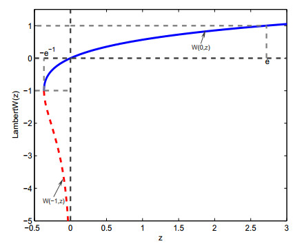
[37]	R. M. Corless, G. H. Gonnet, D. E. G. Hare, D. J. Jeffrey, D. E. Knuth, On the LambertW function, Adv. Comput. Math., 5 (1996), 329–359.

This article has been cited by:

1.	FATMA YAKOUBI, ALI BOUSSAYOUD, BAGHDADI ALOUI, HIND MERZOUK, k-BALANCING NUMBERS AND NEW GENERATING FUNCTIONS WITH SOME SPECIAL NUMBERS AND POLYNOMIALS, 2022, 22, 2068-3049, 929, 10.46939/J.Sci.Arts-22.4-a14
2.	Waleed Mohamed Abd-Elhameed, Amr Kamel Amin, Nasr Anwer Zeyada, Some new identities of a type of generalized numbers involving four parameters, 2022, 7, 2473-6988, 12962, 10.3934/math.2022718
3.	Kalika Prasad, Munesh Kumari, Jagmohan Tanti, Octonions and hyperbolic octonions with the k-balancing and k-Lucas balancing numbers, 2024, 32, 0971-3611, 1281, 10.1007/s41478-023-00716-x

Reader Comments

Your name:*

Email:*
© 2023 the Author(s), licensee AIMS Press. This is an open access article distributed under the terms of the Creative Commons Attribution License (http://creativecommons.org/licenses/by/4.0)