Switching dynamics analysis of forest-pest model describing effects of external periodic disturbance

Yi Yang; Lirong Liu; Changcheng Xiang; Wenjie Qin; Yi Yang; Lirong Liu; Changcheng Xiang; Wenjie Qin

doi:10.3934/mbe.2020239

Mathematical Biosciences and Engineering

2020, Volume 17, Issue 4: 4328-4347. doi: 10.3934/mbe.2020239

Previous Article Next Article

Research article

Switching dynamics analysis of forest-pest model describing effects of external periodic disturbance

1.
College of Computer Science and Engineering, Chongqing Three Gorges University, Chongqing 404100, China
2.
Key Laboratory of Intelligent Information Processing and Control of Chongqing Municipal Institutions of Higher education, Chongqing Three Gorges University, Chongqing 404100, China
3.
School of Mathematics and Statistics, Hubei Minzu University, Enshi 445000, China
4.
Three Gorges Mathematical Research Center, China Three Gorges University, Yichang 443002, China

Received: 18 April 2020 Accepted: 10 June 2020 Published: 19 June 2020

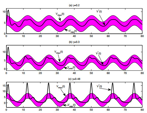
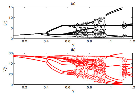
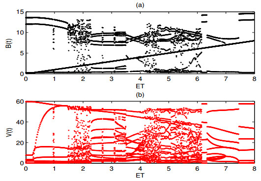
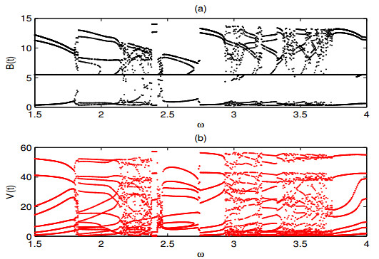
A periodically forced Filippov forest-pest model incorporating threshold policy control and integrated pest management is proposed. It is very natural and reasonable to introduce Filippov non-smooth system into the ecosystem since there were many disadvantageous factors in pest control at fixed time and the threshold control according to state variable showed rewarding characteristics. The main aim of this paper is to quest the association between pests dynamics and system parameters especially the economical threshold ET, the amplitude and frequency of periodic forcing term. From the view of pest control, if the maximum amplitude of the sliding periodic solution does not exceed economic injury level(EIL), the sliding periodic solution is a desired result for pest control. The Filippov forest-pest model exhibits the rich dynamic behaviors including multiple attractors coexistence, period-adding bifurcation, quasi-periodic feature and chaos. At certain frequency of periodic forcing, the varying system initial densities trigger the system state switch between different attractors with diverse amplitudes and periods. Besides, parameters sensitivity analysis shows that the pest could be controlled at a certain level by choosing suitable parameters.
- Filippov forest-pest system,
- integrated pest control,
- periodic forcing,
- bifurcation analysis,
- multiple attractors coexistence
Citation: Yi Yang, Lirong Liu, Changcheng Xiang, Wenjie Qin. Switching dynamics analysis of forest-pest model describing effects of external periodic disturbance[J]. Mathematical Biosciences and Engineering, 2020, 17(4): 4328-4347. doi: 10.3934/mbe.2020239

Related Papers:

Abstract

A periodically forced Filippov forest-pest model incorporating threshold policy control and integrated pest management is proposed. It is very natural and reasonable to introduce Filippov non-smooth system into the ecosystem since there were many disadvantageous factors in pest control at fixed time and the threshold control according to state variable showed rewarding characteristics. The main aim of this paper is to quest the association between pests dynamics and system parameters especially the economical threshold ET, the amplitude and frequency of periodic forcing term. From the view of pest control, if the maximum amplitude of the sliding periodic solution does not exceed economic injury level(EIL), the sliding periodic solution is a desired result for pest control. The Filippov forest-pest model exhibits the rich dynamic behaviors including multiple attractors coexistence, period-adding bifurcation, quasi-periodic feature and chaos. At certain frequency of periodic forcing, the varying system initial densities trigger the system state switch between different attractors with diverse amplitudes and periods. Besides, parameters sensitivity analysis shows that the pest could be controlled at a certain level by choosing suitable parameters.

References

[1]	S. Rinaldi, S. Muratori, Y. Kuznetsov, Multiple attractors, catastrophes and chaos in seasonally perturbed predator-prey communities, B. Math. Biol., 55 (1993), 15-35.
[2]	G. C. Sabin, D. Summers, Chaos in a periodically forced predator-prey ecosystem model, Math. Biosci., 113 (1993), 91-113. doi: 10.1016/0025-5564(93)90010-8
[3]	S. Y. Tang, L. S. Chen, Quasiperiodic solutions and chaos in a periodically forced predator-prey model with age structure for predator, Int. J. Bifurcat. Chaos, 13 (2003), 973-980. doi: 10.1142/S0218127403007011
[4]	S. Gakkhar, R. K. Naji, Chaos in seasonally perturbed ratio-dependent prey-predator system, Chaos Soliton. Fract., 15 (2003), 107-118. doi: 10.1016/S0960-0779(02)00114-5
[5]	G. Q. Sun, Z. Jin, Q. X. Liu, B. L. Li, Rich dynamics in a predator-prey model with both noise and periodic force, Biosystems, 100 (2010), 14-22. doi: 10.1016/j.biosystems.2009.12.003
[6]	T. Caraballo, R. Colucci, X. Han, Non-autonomous dynamics of a semi-kolmogorov population model with periodic forcing, Nonlinear Anal. Real., 31 (2016), 661-680. doi: 10.1016/j.nonrwa.2016.03.007
[7]	S. G. Liu, B. B. Lamberty, J. A. Hicke, R. Vargas, S. Q. Zhao, J. Chen, et al., Simulating the impacts of disturbances on forest carbon cycling in North America: Processes, data, models, and challenges, J. Geophys. Res. Biogeo., 116 (2011), doi: 10.1029/2010JG001585.
[8]	B. D. Cook, P. V. Bolstad, J. G. Martin, F. A. Heinsch, K. J. Davis, W. G. Wang, et al., Using light-use and production efficiency models to predict photosynthesis and net carbon exchange during forest canopy disturbance, Ecosystems, 11 (2008), 26-44.
[9]	R. A. Fleming, J. N. Candau, R. S. Mcalpine, Landscape-scale analysis of interactions between insect defoliation and forest fire in central canada, Climatic Change, 55 (2002), 251-272. doi: 10.1023/A:1020299422491
[10]	B. Chen-Charpentier, M. C. A. Leite, A model for coupling fire and insect outbreak in forests, Ecol. Model., 286 (2014), 26-36. doi: 10.1016/j.ecolmodel.2014.04.008
[11]	M. L. Flint, R. V. D. Bosch, Introduction to Integrated Pest Management, Springer, 1981.
[12]	V. M. Stern, R. F. Smith, R. V. D. Bosch, K. S. Hagen, The integration of chemical and biological control of the spotted alfalfa aphid: The integrated control concept, Hilgardia, 29 (1959), 81-101. doi: 10.3733/hilg.v29n02p081
[13]	J. V. Lenteren, Integrated pest management in protected crops, London: Chapman, Hall, 1995.
[14]	S. Y. Tang, Y. N. Xiao, R. A. Cheke, Multiple attractors of Host-Parasitoid models with integrated pest management strategies: Eradication, persistence and outbreak, Theor. Popul. Biol, 73 (2008), 181-197.
[15]	C. C. Xiang, Y. Yang, Z. Y. Xiang, W. J. Qin, Numerical analysis of discrete switching preypredator model for integrated pest management, Discrete Dyn. Nat. Soc., 2016 (2016), 1-11.
[16]	K. B. Sun, T. H. Zhang, Y. Tian, Dynamics analysis and control optimization of a pest management predator-prey model with an integrated control strategy, Appl. Math. Comput., 292 (2017), 253-271.
[17]	S. Y. Tang, R. A. Cheke, State-dependent impulsive models of integrated pest management (IPM)strategies and their dynamic consequences, J. Math. Biol., 50 (2005), 257-292. doi: 10.1007/s00285-004-0290-6
[18]	S. Y. Tang, R. A. Cheke, Models for integrated pest control and their biological implications, Math. Biosci., 215 (2008), 115-125. doi: 10.1016/j.mbs.2008.06.008
[19]	M. E. M. Meza, A. Bhaya, E. Kaszkurewicz, M. I. da Silveira Costa, Threshold policies control for predator-prey systems using a control Liapunov function approach, Theor. Popul. Biol., 67 (2005), 273-284.
[20]	Z. Y. Xiang, S. Y. Tang, Filippov ratio-dependent prey-predator model with threshold policy control, Abstr. Appl. Anal., 2013(2013), doi:10.1155/2013/280945. doi: 10.1155/2013/280945
[21]	L. R. Liu, C. C. Xiang, G. Y. Tang, Dynamics analysis of periodically forced Filippov Holling II prey-predator model with integrated pest control, IEEE Access, 2019(2019), doi: 10.1109/ACCESS.2019.2934600. doi: 10.1109/ACCESS.2019.2934600
[22]	G. Y. Tang, W. J. Qin, S. Y. Tang, Complex dynamics and switching transients in periodically forced Filippov prey-predator system, Chaos Soliton. Fract., 61 (2014), 13-23. doi: 10.1016/j.chaos.2014.02.002
[23]	W. J. Qin, X. W. Tan, X. T. Shi, J. H. Chen, X. Z. Liu, Dynamics and bifurcation analysis of a Filippov predator-prey ecosystem in a seasonally fluctuating environment, Int. J. Bifurcat. Chaos, 29 (2019), doi: 10.1142/S0218127419500202.
[24]	L. R. Liu, C. C. Xiang, G. Y. Tang, Y. Fu, Sliding dynamics of a Filippov forest-pest model with threshold policy control, Complexity, 2019 (2019), doi:10.1155/2019/2371838. doi: 10.1155/2019/2371838
[25]	A. F. Filippov, Equations with the right-hand side continuous in x and discontinuous in t, Differential equations with discontinuous righthand sides, Springer Netherlands, 1988.
[26]	Y. A. Kuznetsov, S. Rinaldi, A. Gragnani, One-parameter bifurcations in planar Filippov systems, Int. J. Bifurcat. Chaos, 13 (2003), 2157-2188. doi: 10.1142/S0218127403007874
[27]	B. Brogliato, Nonsmooth mechanics, New York: Springer Verlag, 1999.
[28]	B. Brogliato, Impacts in mechanical systems: analysis and modelling, Springer Science and Business Media, 2000.
[29]	K. Gupta, S. Gakkhar, The Filippov approach for predator-prey system involving mixed type of functional responses, Dynam. Part. Differ. Eq., 2016 (2016), doi:10.1007/s12591-016-0322-x. doi: 10.1007/s12591-016-0322-x
[30]	W. J. Qin, X. W. Tan, M. Tosato, X. Z. Liu, Threshold control strategy for a non-smooth Filippov ecosystem with group defense, Appl. Math. Comput., 362 (2019), 124532.
[31]	X. H. Zhang, S. Y. Tang, Existence of multiple sliding segments and bifurcation analysis of Filippov prey-predator model, Appl. Math. Comput., 239 (2014), 265-284.
[32]	H. Zhou, X. Wang, S. Y. Tang, Global dynamics of non-smooth Filippov pest-natural enemy system with constant releasing rate, Math. Biosci. Eng., 16 (2019), 7327-7361. doi: 10.3934/mbe.2019366
[33]	F. H.Yang, W. Zhang, J. Wang, Sliding bifurcations and chaos induced by dry friction in a braking system, Chaos Soliton. Fract., 40 (2009), 1060-1075. doi: 10.1016/j.chaos.2007.08.079
[34]	V. Utkin, J. Guldner, J. Shi, Sliding mode control in electro-mechanical systems, Boca Raton, FL, USA: CRC Press, 2009.
[35]	Y. N. Xiao, S. Y. Tang, J. H. Wu, Media impact switching surface during an infectious disease outbreak, Sci. Rep-Uk., 5 (2015), doi: 10.1038/srep07838.
[36]	A. L. Wang, Y. N. Xiao, H. P.Zhu, Dynamics of a Filippov epidemic model with limited hospital beds, Math. Biosci. Eng., 15 (2018), 739-764.
[37]	A. L. Wang, Y. N. Xiao, R. Smith, Multiple equilibria in a non-smooth epidemic model with medical-resource constraints, B. Math. Biol., 81 (2019), 963-994. doi: 10.1007/s11538-018-00544-2
[38]	Y. Yang, X. F. Liao, Filippov Hindmarsh-Rose neuronal model with threshold policy control, IEEE T. Neur. Net. Lear., 30 (2018), 306-311.
[39]	M. Guardia, S. J. Hogan, T. M. Seara, An analytical approach to codimension-2 sliding bifurcations in the dry-friction oscillator, SIAM. J. Appl. Dyn. Syst., 9 (2010), 769-798. doi: 10.1137/090766826
[40]	J. C. Sprott, X. Wang, G. R. Chen, Coexistence of point, periodic and strange attractors, Int. J. Bifurcat. Chaos, 23 (2013), doi: 10.1142/S0218127413500934.
[41]	A. Grinsted, J. C. Moore, S. Jevrejeva, Application of the cross wavelet transform and wavelet coherence to geophysical time series, Nonlinear Proc. Geoph., 11 (2004), 561-566. doi: 10.5194/npg-11-561-2004
[42]	C. Torrence, G. P. Compo, A practical guide to wavelet analysis, B. Am. Meteorol Soc., 79 (1998), 61-78.
[43]	Q. L. Yan, S. Y. Tang, Z. Jin, Y. N. Xiao, Identifying risk factors of a (H7N9) outbreak by wavelet analysis and generalized estimating equation, Inter. J. Env. Res. Pub. Heal., 16 (2019), 1-13.

Reader Comments

Your name:*

Email:*
© 2020 the Author(s), licensee AIMS Press. This is an open access article distributed under the terms of the Creative Commons Attribution License (http://creativecommons.org/licenses/by/4.0)