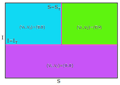
This paper proposes a non-smooth human influenza model with logistic source to describe the impact on media coverage and quarantine of susceptible populations of the human influenza transmission process. First, we choose two thresholds $ I_{T} $ and $ S_{T} $ as a broken line control strategy: Once the number of infected people exceeds $ I_{T} $, the media influence comes into play, and when the number of susceptible individuals is greater than $ S_{T} $, the control by quarantine of susceptible individuals is open. Furthermore, by choosing different thresholds $ I_{T} $ and $ S_{T} $ and using Filippov theory, we study the dynamic behavior of the Filippov model with respect to all possible equilibria. It is shown that the Filippov system tends to the pseudo-equilibrium on sliding mode domain or one endemic equilibrium or bistability endemic equilibria under some conditions. The regular/virtulal equilibrium bifurcations are also given. Lastly, numerical simulation results show that choosing appropriate threshold values can prevent the outbreak of influenza, which implies media coverage and quarantine of susceptible individuals can effectively restrain the transmission of influenza. The non-smooth system with logistic source can provide some new insights for the prevention and control of human influenza.
Citation: Guodong Li, Wenjie Li, Ying Zhang, Yajuan Guan. Sliding dynamics and bifurcations of a human influenza system under logistic source and broken line control strategy[J]. Mathematical Biosciences and Engineering, 2023, 20(4): 6800-6837. doi: 10.3934/mbe.2023293
This paper proposes a non-smooth human influenza model with logistic source to describe the impact on media coverage and quarantine of susceptible populations of the human influenza transmission process. First, we choose two thresholds $ I_{T} $ and $ S_{T} $ as a broken line control strategy: Once the number of infected people exceeds $ I_{T} $, the media influence comes into play, and when the number of susceptible individuals is greater than $ S_{T} $, the control by quarantine of susceptible individuals is open. Furthermore, by choosing different thresholds $ I_{T} $ and $ S_{T} $ and using Filippov theory, we study the dynamic behavior of the Filippov model with respect to all possible equilibria. It is shown that the Filippov system tends to the pseudo-equilibrium on sliding mode domain or one endemic equilibrium or bistability endemic equilibria under some conditions. The regular/virtulal equilibrium bifurcations are also given. Lastly, numerical simulation results show that choosing appropriate threshold values can prevent the outbreak of influenza, which implies media coverage and quarantine of susceptible individuals can effectively restrain the transmission of influenza. The non-smooth system with logistic source can provide some new insights for the prevention and control of human influenza.

| [1] |
D. M. Morens, A. S. Fauci, The 1918 influenza pandemic: insights for the 21st century, J. Infect. Dis., 195 (2007), 1018–1028. https://doi.org/10.1086/511989 doi: 10.1086/511989

|
| [2] | M. Babakir-Mina, S. Dimonte, M. Ciccozzi, C. F. Perno, M. Ciotti, The novel swine-origin H1N1 influenza A virus riddle: is it a domestic bird H1N1-derived virus, New Microbiol., 33 (2010), 77–81. |
| [3] | F. Ferrajoli, Influenza in the Italian army & the recent Asiatic pandemic in the group. Ⅱ. The so-called Asiatic flu pandemic in the army, G. Med. Mil., 108 (1958), 309–337. |
| [4] |
T. D. Rozen, Daily persistent headache after a viral illness during a worldwide pandemic may not be a new occurrence: Lessons from the 1890 Russian/Asiatic flu, Cephalalgia, 40 (2020), 1406–1409. https://doi.org/10.1177/0333102420965132 doi: 10.1177/0333102420965132
|
| [5] |
A. Sutter, M. Vaswani, P. Denice, K. H. Choi, J. Bouchard, V. M. Esses, Ageism toward older adults during the COVID‐19 pandemic: intergenerational conflict and support, J. Soc. Issues, 2022 (2022). https://doi.org/10.1111/josi.12554 doi: 10.1111/josi.12554
|
| [6] |
S. Saha, G. Samanta, J. J. Nieto, Impact of optimal vaccination and social distancing on COVID-19 pandemic, Math. Comput. Simul., 200 (2022), 285–314. https://doi.org/10.1016/j.matcom.2022.04.025 doi: 10.1016/j.matcom.2022.04.025
|
| [7] |
D. K. Chu, E. A. Akl, S. Duda, K. Solo, S. Yaacoub, H. J. Schünemann, et al., Physical distancing, face masks, and eye protection to prevent person-to-person transmission of SARS-CoV-2 and COVID-19: a systematic review and meta-analysis, Lancet, 395 (2020), 1973–1987. https://doi.org/10.1016/S0140-6736(20)31142-9 doi: 10.1016/S0140-6736(20)31142-9
|
| [8] |
H. W. Berhe, O. D. Makinde, Computational modelling and optimal control of measles epidemic in human population, Biosystems, 190 (2020), 104102. https://doi.org/10.1016/j.biosystems.2020.104102 doi: 10.1016/j.biosystems.2020.104102
|
| [9] |
H. W. Berhe, O. D. Makinde, D. M. Theuri, Optimal control and cost-effectiveness analysis for dysentery epidemic model, Appl. Math. Inf. Sci., 12 (2018), 1183–1195. https://doi.org/10.18576/amis/120613 doi: 10.18576/amis/120613
|
| [10] |
A. Omame, N. Sene, I. Nometa, C. I. Nwakanma, E. U. Nwafor, N. O. Iheonu, et al., Analysis of COVID‐19 and comorbidity co‐infection model with optimal control, Optim. Control. Appl. Methods, 42 (2021), 1568–1590. https://doi.org/10.1002/oca.2748 doi: 10.1002/oca.2748
|
| [11] |
A. Babaei, M. Ahmadi, H. Jafari, A. Liya, A mathematical model to examine the effect of quarantine on the spread of coronavirus, Chaos, Solitons Fractals, 142 (2021), 110418. https://doi.org/10.1016/j.chaos.2020.110418 doi: 10.1016/j.chaos.2020.110418
|
| [12] |
M. Z. Ndii, Y. A. Adi, Understanding the effects of individual awareness and vector controls on malaria transmission dynamics using multiple optimal control, Chaos, Solitons Fractals, 153 (2021), 111476. https://doi.org/10.1016/j.chaos.2021.111476 doi: 10.1016/j.chaos.2021.111476
|
| [13] |
W. Li, J. Ji, L. Huang, J. Wang, Bifurcations and dynamics of a plant disease system under non-smooth control strategy, Nonlinear Dyn., 99 (2020), 3351–3371. https://doi.org/10.1007/s11071-020-05464-2 doi: 10.1007/s11071-020-05464-2
|
| [14] |
W. Li, J. Ji, L. Huang, Dynamics of a controlled discontinuous computer worm system, Proc. Amer. Math. Soc., 148 (2020), 4389–4403. https://doi.org/10.1090/proc/15095 doi: 10.1090/proc/15095
|
| [15] |
J. Deng, S. Tang, H. Shu, Joint impacts of media, vaccination and treatment on an epidemic Filippov model with application to COVID-19, J. Theor. Biol., 523 (2021), 110698. https://doi.org/10.1016/j.jtbi.2021.110698 doi: 10.1016/j.jtbi.2021.110698
|
| [16] |
T. Li, Y. Guo, Modeling and optimal control of mutated COVID-19 (Delta strain) with imperfect vaccination, Chaos, Solitons Fractals, 156 (2022), 111825. https://doi.org/10.1016/j.chaos.2022.111825 doi: 10.1016/j.chaos.2022.111825
|
| [17] |
A. Kouidere, L. E. L. Youssoufi, H. Ferjouchia, O. Balatif, M. Rachik, Optimal control of mathematical modeling of the spread of the COVID-19 pandemic with highlighting the negative impact of quarantine on diabetics people with cost-effectiveness, Chaos, Solitons Fractals, 145 (2021), 110777. https://doi.org/10.1016/j.chaos.2021.110777 doi: 10.1016/j.chaos.2021.110777
|
| [18] |
C. A. K. Kwuimy, F. Nazari, X. Jiao, P. Rohani, C. Nataraj, Nonlinear dynamic analysis of an epidemiological model for COVID-19 including public behavior and government action, Nonlinear Dyn., 101 (2020), 1545–1559. https://doi.org/10.1007/s11071-020-05815-z doi: 10.1007/s11071-020-05815-z
|
| [19] |
M. A. Khan, A. Atangana, E. Alzahrani, The dynamics of COVID-19 with quarantined and isolation, Adv. Differ. Equations, 2020 (2020), 1–22. https://doi.org/10.1186/s13662-020-02882-9 doi: 10.1186/s13662-020-02882-9
|
| [20] |
A. Aleta, D. Martín-Corral, A. P. Piontti, M. Ajelli, M. Litvinova, M. Chinazzi, et al., Modelling the impact of testing, contact tracing and household quarantine on second waves of COVID-19, Nat. Hum. Behav., 4 (2020), 964–971. https://doi.org/10.1038/s41562-020-0931-9 doi: 10.1038/s41562-020-0931-9
|
| [21] |
Y. Yuan, N. Li, Optimal control and cost-effectiveness analysis for a COVID-19 model with individual protection awareness, Physica A, 603 (2022), 127804. https://doi.org/10.1016/j.physa.2022.127804 doi: 10.1016/j.physa.2022.127804
|
| [22] |
A. Wang, Y. Xiao, Sliding bifurcation and global dynamics of a Filippov epidemic model with vaccination, Int. J. Bifurcation Chaos, 23 (2013), 1350144. https://doi.org/10.1142/S0218127413501447 doi: 10.1142/S0218127413501447
|
| [23] |
M. De la Sen, A. Ibeas, On an SE(Is)(Ih)AR epidemic model with combined vaccination and antiviral controls for COVID-19 pandemic, Adv. Differ. Equations, 2021 (2021), 1–30. https://doi.org/10.1186/s13662-021-03248-5 doi: 10.1186/s13662-021-03248-5
|
| [24] |
O. Agossou, M. N. Atchadé, A. M. Djibril, Modeling the effects of preventive measures and vaccination on the COVID-19 spread in Benin Republic with optimal control, Results Phys., 31 (2021), 104969. https://doi.org/10.1016/j.rinp.2021.104969 doi: 10.1016/j.rinp.2021.104969
|
| [25] |
C. Chen, N. S. Chong, R. Smith, A Filippov model describing the effects of media coverage and quarantine on the spread of human influenza, Math. Biosci., 296 (2018), 98–112. https://doi.org/10.1016/j.mbs.2017.12.002 doi: 10.1016/j.mbs.2017.12.002
|
| [26] |
J. Cui, Y. Sun, H. Zhu, The impact of media on the control of infectious diseases, J. Dyn. Differ. Equations, 20 (2008), 31–53. https://doi.org/10.1007/s10884-007-9075-0 doi: 10.1007/s10884-007-9075-0
|
| [27] |
J. M. Tchuenche, N. Dube, C. P. Bhunu, R. J. Smith, C. T. Bauch, The impact of media coverage on the transmission dynamics of human influenza, BMC Public Health, 11 (2011), 1–14. https://doi.org/10.1186/1471-2458-11-S1-S5 doi: 10.1186/1471-2458-11-S1-S5
|
| [28] |
Y. Xiao, S. Tang, J. Wu, Media impact switching surface during an infectious disease outbreak, Sci. Rep., 5 (2015), 1–9. https://doi.org/10.1038/srep07838 doi: 10.1038/srep07838
|
| [29] |
Y. Xiao, T. Zhao, S. Tang, Dynamics of an infectious diseases with media/psychology induced non-smooth incidence, Math. Biosci. Eng., 10 (2013), 445. https://doi.org/10.3934/mbe.2013.10.445 doi: 10.3934/mbe.2013.10.445
|
| [30] |
W. Li, Y. Chen, L. Huang, J. Wang, Global dynamics of a Filippov predator-prey model with two thresholds for integrated pest management, Chaos, Solitons Fractals, 157 (2022), 111881. https://doi.org/10.1016/j.chaos.2022.111881 doi: 10.1016/j.chaos.2022.111881
|
| [31] |
C. Chen, C. Li, Y. Kang, Modelling the effects of cutting off infected branches and replanting on fire-blight transmission using Filippov systems, J. Theor. Biol., 439 (2018), 127–140. https://doi.org/10.3917/nrt.401.0127 doi: 10.3917/nrt.401.0127
|
| [32] |
W. Zhou, Y. Xiao, J. M. Heffernan, A two-thresholds policy to interrupt transmission of West Nile Virus to birds, J. Theor. Biol., 463 (2019), 22–46. https://doi.org/10.1016/j.jtbi.2018.12.013 doi: 10.1016/j.jtbi.2018.12.013
|
| [33] |
C. Dong, C. Xiang, W. Qin, Y. Yang, Global dynamics for a Filippov system with media effects, Math. Biosci. Eng., 19 (2022), 2835–2852. https://doi.org/10.3934/mbe.2022130 doi: 10.3934/mbe.2022130
|
| [34] |
W. Li, J. Ji, L. Huang, Z. Guo, Global dynamics of a controlled discontinuous diffusive SIR epidemic system, Appl. Math. Lett., 121 (2021), 107420 https://doi.org/10.1016/j.aml.2021.107420 doi: 10.1016/j.aml.2021.107420
|
| [35] |
W. Li, J. Ji, L. Huang, L. Zhang, Global dynamics and control of malicious signal transmission in wireless sensor networks, Nonlinear Anal. Hybrid Syst., 48 (2023), 101324. https://doi.org/10.1016/j.nahs.2022.101324 doi: 10.1016/j.nahs.2022.101324
|
| [36] |
Z. Cai, L. Huang, Generalized Lyapunov approach for functional differential inclusions, Automatica, 113 (2020), 108740. https://doi.org/10.1016/j.automatica.2019.108740 doi: 10.1016/j.automatica.2019.108740
|
| [37] |
W. Li, Y. Zhang, L. Huang, Dynamics analysis of a predator–prey model with nonmonotonic functional response and impulsive control, Math. Comput. Simul., 204 (2023), 529–555. https://doi.org/10.1016/j.matcom.2022.09.002 doi: 10.1016/j.matcom.2022.09.002
|
| [38] |
W. Li, J. Ji, L. Huang, Global dynamics analysis of a water hyacinth fish ecological system under impulsive control, J. Franklin Inst., 359 (2022), 10628–10652. https://doi.org/10.1016/j.jfranklin.2022.09.030 doi: 10.1016/j.jfranklin.2022.09.030
|
| [39] |
Z. Cai, L. Huang, Z. Wang, Fixed/Preassigned-time stability of time-varying nonlinear system with discontinuity: application to Chua's circuit, IEEE Trans. Circuits Syst. II Express Briefs, 69 (2022), 2987–2991. https://doi.org/10.1109/TCSII.2022.3166776 doi: 10.1109/TCSII.2022.3166776
|
| [40] |
Z. Cai, L. Huang, Z. Wang, Novel fixed-time stability criteria for discontinuous nonautonomous systems: Lyapunov method with indefinite derivative, IEEE Trans. Cybern., 52 (2020), 4286–4299. https://doi.org/10.1109/TCYB.2020.3025754 doi: 10.1109/TCYB.2020.3025754
|
| [41] |
H. Tu, X. Wang, S. Tang, Exploring COVID-19 transmission patterns and key factors during epidemics caused by three major strains in Asia, J. Theor. Biol., 557 (2023), 111336. https://doi.org/10.1016/j.jtbi.2022.111336 doi: 10.1016/j.jtbi.2022.111336
|
| [42] |
J. Wang, Z. Huang, Z. Wu, J. Cao, H. Shen, Extended dissipative control for singularly perturbed PDT switched systems and its application, Trans. Circuits Syst. I Regul. Pap., 67 (2020), 5281–5289. https://doi.org/10.1109/TCSI.2020.3022729 doi: 10.1109/TCSI.2020.3022729
|
| [43] |
W. Li, J. Ji, L. Huang, Y. Zhang, Complex dynamics and impulsive control of a chemostat model under the ratio threshold policy, Chaos, Solitons Fractals, 167 (2023), 113077. https://doi.org/10.1016/j.chaos.2022.113077 doi: 10.1016/j.chaos.2022.113077
|
| [44] |
J. Li, Q. Zhu, Stability of neutral stochastic delayed systems with switching and distributed-delay dependent impulses, Nonlinear Anal. Hybrid Syst., 47 (2023), 101279. https://doi.org/10.1016/j.nahs.2022.101279 doi: 10.1016/j.nahs.2022.101279
|
| [45] |
C. Chen, P. Wang, L. Zhang, A two-thresholds policy for a Filippov model in combating influenza, J. Math. Biol., 81 (2020), 435–461. https://doi.org/10.1007/s00285-020-01514-w doi: 10.1007/s00285-020-01514-w
|
| [46] |
Y. A. Kuznetsov, S. Rinaldi, A. Gragnani, One-parameter bifurcations in planar Filippov systems, Int. J. Bifurcation Chaos, 13 (2003), 2157–2188. https://doi.org/10.1142/S0218127403007874 doi: 10.1142/S0218127403007874
|
| [47] |
N. S. Chong, B. Dionne, R. Smith, An avian-only Filippov model incorporating culling of both susceptible and infected birds in combating avian influenza, J. Math. Biol., 73 (2016), 751–784. https://doi.org/10.1007/s00285-016-0971-y doi: 10.1007/s00285-016-0971-y
|


Figures(10) / Tables(3)

Guodong Li, Wenjie Li, Ying Zhang, Yajuan Guan. Sliding dynamics and bifurcations of a human influenza system under logistic source and broken line control strategy[J]. Mathematical Biosciences and Engineering, 2023, 20(4): 6800-6837. doi: 10.3934/mbe.2023293


 DownLoad: