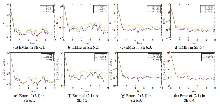
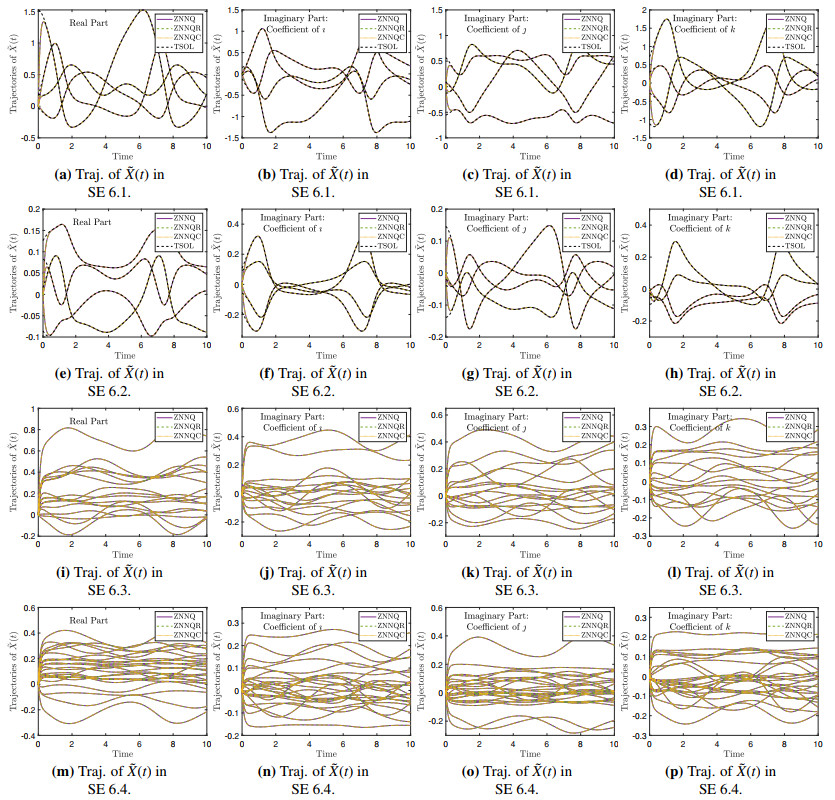
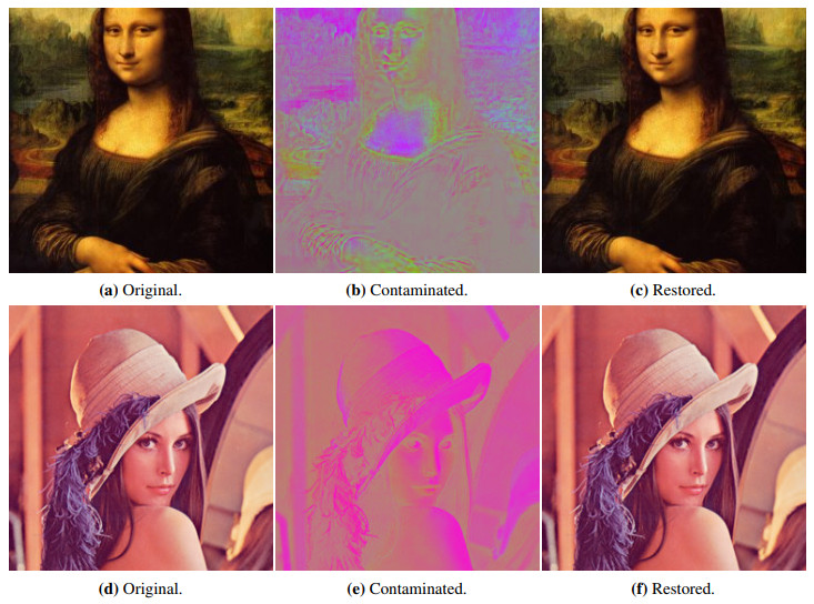
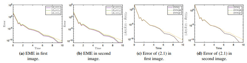
The importance of quaternions in a variety of fields, such as physics, engineering and computer science, renders the effective solution of the time-varying quaternion matrix linear equation (TV-QLME) an equally important and interesting task. Zeroing neural networks (ZNN) have seen great success in solving TV problems in the real and complex domains, while quaternions and matrices of quaternions may be readily represented as either a complex or a real matrix, of magnified size. On that account, three new ZNN models are developed and the TV-QLME is solved directly in the quaternion domain as well as indirectly in the complex and real domains for matrices of arbitrary dimension. The models perform admirably in four simulation experiments and two practical applications concerning color restoration of images.
Citation: Vladislav N. Kovalnogov, Ruslan V. Fedorov, Denis A. Demidov, Malyoshina A. Malyoshina, Theodore E. Simos, Vasilios N. Katsikis, Spyridon D. Mourtas, Romanos D. Sahas. Zeroing neural networks for computing quaternion linear matrix equation with application to color restoration of images[J]. AIMS Mathematics, 2023, 8(6): 14321-14339. doi: 10.3934/math.2023733
The importance of quaternions in a variety of fields, such as physics, engineering and computer science, renders the effective solution of the time-varying quaternion matrix linear equation (TV-QLME) an equally important and interesting task. Zeroing neural networks (ZNN) have seen great success in solving TV problems in the real and complex domains, while quaternions and matrices of quaternions may be readily represented as either a complex or a real matrix, of magnified size. On that account, three new ZNN models are developed and the TV-QLME is solved directly in the quaternion domain as well as indirectly in the complex and real domains for matrices of arbitrary dimension. The models perform admirably in four simulation experiments and two practical applications concerning color restoration of images.

| [1] | W. R. Hamilton, On a new species of imaginary quantities, connected with the theory of quaternions, P. Roy. Irish Acad. (1836–1869), 2 (1840), 424–434. |
| [2] |
B. L. Van Der Waerden, Hamilton's discovery of quaternions, Math. Magazine, 49 (1976), 227–234. https://doi.org/10.1080/0025570X.1976.11976586 doi: 10.1080/0025570X.1976.11976586

|
| [3] | K. Shoemake, Animating rotation with quaternion curves, In: Proceedings of the 12th annual conference on Computer graphics and interactive techniques, 1985,245–254. |
| [4] |
R. Goldman, Understanding quaternions, Graph. Models, 73 (2011), 21–49. https://doi.org/10.1016/j.gmod.2010.10.004 doi: 10.1016/j.gmod.2010.10.004
|
| [5] | M. Joldeş, J. M. Muller, Algorithms for manipulating quaternions in floating-point arithmetic, In: 2020 IEEE 27th Symposium on Computer Arithmetic (ARITH), IEEE, 2020, 48–55. |
| [6] | A. Szynal-Liana, I. Włoch, Generalized commutative quaternions of the Fibonacci type, Boletín de la Sociedad Matemática Mexicana, 28 (2022), 1. |
| [7] |
D. Pavllo, C. Feichtenhofer, M. Auli, D. Grangier, Modeling human motion with quaternion-based neural networks, Int. J. Comput. Vision, 128 (2020), 855–872. https://doi.org/10.1007/s11263-019-01207-y doi: 10.1007/s11263-019-01207-y
|
| [8] | J. Funda, R. H. Taylor, R. P. Paul, On homogeneous transforms, quaternions, and computational efficiency, IEEE T. Robot. Autom., 6 (1990), 382–388. |
| [9] | M. Gouasmi, Robot kinematics, using dual quaternions, IAES Int. J. Robot. Autom., 1 (2012), 13. |
| [10] | J. S. Yuan, Closed-loop manipulator control using quaternion feedback, IEEE J. Robot. Autom., 4 (1988), 434–440. |
| [11] |
E. Özgür, Y. Mezouar, Kinematic modeling and control of a robot arm using unit dual quaternions, Robot. Autonom. Syst., 77 (2016), 66–73. https://doi.org/10.1016/j.robot.2015.12.005 doi: 10.1016/j.robot.2015.12.005
|
| [12] | A. R. Klumpp, Singularity-free extraction of a quaternion from a direction-cosine matrix, J. Spacecraft Rockets, 13 (1976), 754–755. |
| [13] | B. Wie, P. M. Barba, Quaternion feedback for spacecraft large angle maneuvers, J. Guid. Control Dynam., 8 (1985), 360–365. |
| [14] | A. M. S. Goodyear, P. Singla, D. B. Spencer, Analytical state transition matrix for dual-quaternions for spacecraft pose estimation, In: AAS/AIAA Astrodynamics Specialist Conference, 2019, Univelt Inc., 2020,393–411. |
| [15] | Quaternionic quantum mechanics and quantum fields, Phys. Today, 49 (1996), 58. https://doi.org/10.1063/1.2807466 |
| [16] |
H. Kaiser, E. A. George, S. A. Werner, Neutron interferometric search for quaternions in quantum mechanics, Phys. Rev. A, 29 (1984), 2276. https://doi.org/10.1103/PhysRevA.29.2276 doi: 10.1103/PhysRevA.29.2276
|
| [17] |
A. J. Davies, B. H. J. McKellar, Nonrelativistic quaternionic quantum mechanics in one dimension, Phys. Rev. A, 40 (1989), 4209. https://doi.org/10.1103/PhysRevB.40.4209 doi: 10.1103/PhysRevB.40.4209
|
| [18] |
A. J. Davies, B. H. J. McKellar, Observability of quaternionic quantum mechanics, Phys. Rev. A, 46 (1992), 3671. https://doi.org/10.1103/PhysRevA.46.3671 doi: 10.1103/PhysRevA.46.3671
|
| [19] |
S. Giardino, Quaternionic quantum mechanics in real Hilbert space, J. Geom. Phys., 158 (2020), 103956. https://doi.org/10.1016/j.geomphys.2020.103956 doi: 10.1016/j.geomphys.2020.103956
|
| [20] |
M. E. Kansu, Quaternionic representation of electromagnetism for material media, Int. J. Geom. Methods M., 16 (2019), 1950105. https://doi.org/10.1142/S0219887819501056 doi: 10.1142/S0219887819501056
|
| [21] | S. Demir, M. Tanışlı, N. Candemir, Hyperbolic quaternion formulation of electromagnetism, Adv. Appl. Clifford Al., 20 (2010), 547–563. |
| [22] |
I. Frenkel, M. Libine, Quaternionic analysis, representation theory and physics, Adv. Math., 218 (2008), 1806–1877. https://doi.org/10.1016/j.aim.2008.03.021 doi: 10.1016/j.aim.2008.03.021
|
| [23] | Z. H. Weng, Field equations in the complex quaternion spaces, Adv. Math. Phys., 2014. |
| [24] | V. G. Kravchenko, V. V. Kravchenko, Quaternionic factorization of the Schrödinger operator and its applications to some first-order systems of mathematical physics, J. Phys. A-Math. Gen., 36 (2003), 11285. |
| [25] |
R. Ghiloni, V. Moretti, A. Perotti, Continuous slice functional calculus in quaternionic Hilbert spaces, Rev. Math. Phys., 25 (2013), 1350006. https://doi.org/10.1142/S0129055X13500062 doi: 10.1142/S0129055X13500062
|
| [26] | J. Groß, G. Trenkler, S. O. Troschke, Quaternions: Further contributions to a matrix oriented approach, Linear Algebra Appl, 326 (2001), 205–213. |
| [27] | L. Xiao, S. Liu, X. Wang, Y. He, L. Jia, Y. Xu, Zeroing neural networks for dynamic quaternion-valued matrix inversion, IEEE T. Ind. Inform., 18 (2022), 1562–1571. |
| [28] | R. W. Farebrother, J. Groß, S. O. Troschke, Matrix representation of quaternions, Linear Algebra Appl, 362 (2003), 251–255. |
| [29] | F. Zhang, Quaternions and matrices of quaternions, Linear Algebra Appl., 251 (1997), 21–57. |
| [30] | L. Xiao, W. Huang, X. Li, F. Sun, Q. Liao, L. Jia, et al., ZNNs with a varying-parameter design formula for dynamic Sylvester quaternion matrix equation, IEEE T. Neural Network. Learn. Syst., 1–11. |
| [31] | L. Xiao, P. Cao, W. Song, L. Luo, W. Tang, A fixed-time noise-tolerance ZNN model for time-variant inequality-constrained quaternion matrix least-squares problem, IEEE T. Neural Network. Learn. Syst., 1–10. |
| [32] | G. Du, Y. Liang, B. Gao, S. A. Otaibi, D. Li, A cognitive joint angle compensation system based on self-feedback fuzzy neural network with incremental learning, IEEE T. Ind. Inform., 17 (2021), 2928–2937. |
| [33] | L. Xiao, Y. Zhang, W. Huang, L. Jia, X. Gao, A dynamic parameter noise-tolerant zeroing neural network for time-varying quaternion matrix equation with applications, IEEE T. Neural Network. Learn. Syst., 1–10. |
| [34] | Y. Zhang, S. S. Ge, Design and analysis of a general recurrent neural network model for time-varying matrix inversion, IEEE T. Neural Network., 16 (2005), 1477–1490. |
| [35] |
J. Jin, J. Zhu, L. Zhao, L. Chen, A fixed-time convergent and noise-tolerant zeroing neural network for online solution of time-varying matrix inversion, Appl. Soft Comput., 130 (2022), 109691. https://doi.org/10.1016/j.asoc.2022.109691 doi: 10.1016/j.asoc.2022.109691
|
| [36] |
T. E. Simos, V. N. Katsikis, S. D. Mourtas, P. S. Stanimirović, D. Gerontitis, A higher-order zeroing neural network for pseudoinversion of an arbitrary time-varying matrix with applications to mobile object localization, Information Sciences, 600 (2022), 226–238. https://doi.org/10.1016/j.ins.2022.03.094 doi: 10.1016/j.ins.2022.03.094
|
| [37] | W. Jiang, C. L. Lin, V. N. Katsikis, S. D. Mourtas, P. S. Stanimirović, T. E. Simos, Zeroing neural network approaches based on direct and indirect methods for solving the Yang–Baxter-like matrix equation, Mathematics, 10 (2022), 1950. |
| [38] | T. E. Simos, V. N. Katsikis, S. D. Mourtas, P. S. Stanimirović, Unique non-negative definite solution of the time-varying algebraic Riccati equations with applications to stabilization of LTV systems, Math. Comput. Simulat., 202 (2022), 164–180. |
| [39] | T. E. Simos, V. N. Katsikis, S. D. Mourtas, P. S. Stanimirović, Finite-time convergent zeroing neural network for solving time-varying algebraic Riccati equations, J. Franklin I., 359 (2022), 10867–10883. |
| [40] |
S. D. Mourtas, V. N. Katsikis, Exploiting the Black-Litterman framework through error-correction neural networks, Neurocomputing, 498 (2022), 43–58. https://doi.org/10.1016/j.neucom.2022.05.036 doi: 10.1016/j.neucom.2022.05.036
|
| [41] | V. N. Kovalnogov, R. V. Fedorov, D. A. Generalov, A. V. Chukalin, V. N. Katsikis, S. D. Mourtas, et al., Portfolio insurance through error-correction neural networks, Mathematics, 10 (2022), 3335. |
| [42] | J. Jin, W. Chen, C. Chen, L. Chen, Z. Tang, L. Chen, et al., A predefined fixed-time convergence ZNN and its applications to time-varying quadratic programming solving and dual-arm manipulator cooperative trajectory tracking, IEEE T. Ind. Inform., 1–12. |
| [43] |
Y. Liu, K. Liu, G. Wang, Z. Sun, L. Jin, Noise-tolerant zeroing neurodynamic algorithm for upper limb motion intention-based human-robot interaction control in non-ideal conditions, Expert Syst. Appl., 213 (2023), 118891. https://doi.org/10.1016/j.eswa.2022.118891 doi: 10.1016/j.eswa.2022.118891
|
| [44] | D. Chen, S. Li, Q. Wu, A novel supertwisting zeroing neural network with application to mobile robot manipulators, IEEE T. Neural Network. Learn. Syst., 32 (2021), 1776–1787. |
| [45] | V. N. Katsikis, S. D. Mourtas, P. S. Stanimirović, S. Li, X. Cao, Time-varying mean-variance portfolio selection problem solving via LVI-PDNN, Comput. Oper. Res., 138 (2022), 105582. |
| [46] | V. N. Katsikis, S. D. Mourtas, P. S. Stanimirović, S. Li, X. Cao, Time-varying minimum-cost portfolio insurance problem via an adaptive fuzzy-power LVI-PDNN, Appl. Math. Comput., 441 (2023), 127700. |
| [47] | W. Chen, J. Jin, D. Gerontitis, L. Qiu, J. Zhu, Improved recurrent neural networks for text classification and dynamic Sylvester equation solving, Neural Processing Lett., 1–30. |
Figures(5) / Tables(2)

Vladislav N. Kovalnogov, Ruslan V. Fedorov, Denis A. Demidov, Malyoshina A. Malyoshina, Theodore E. Simos, Vasilios N. Katsikis, Spyridon D. Mourtas, Romanos D. Sahas. Zeroing neural networks for computing quaternion linear matrix equation with application to color restoration of images[J]. AIMS Mathematics, 2023, 8(6): 14321-14339. doi: 10.3934/math.2023733


 DownLoad: