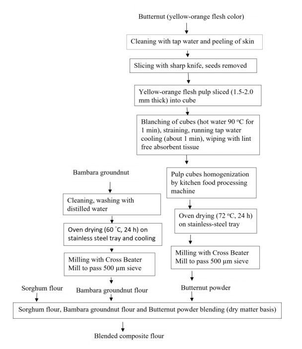
The refined sorghum flour (SF) used is limited in fiber and micronutrients because of bran removal during milling, and protein digestibility is poor due to kafrin crosslinking. In this research, the effects of Bambara groundnut (BG) (15%, 25%, 35%) and butternut (BU) powder (23%) blending on SF were investigated, using 100% SF as a control. The proximate, mineral, beta-carotene and folic acid compositions of the flour mix were determined. As the BG levels increased, the protein, fat, fiber, and ash contents increased significantly (p < 0.05), ranging between 8.62–14.19%, 2.36–3.38%, 1.37–3.04% and 0.87–2.19%, respectively. The iron, zinc, calcium and phosphorus contents in mg/100 g were 3.43–5.08, 2.96–3.74, 80.00–106.67 and 150.63–594.53, respectively. The beta-carotene (mg/100 g) and folic acid (μg/100 g) contents were < 0.01–0.63 and 0.75–1.42, respectively. The mineral, beta-carotene and folic acid contents of the flour mix varied significantly (p < 0.05) from the control. The pro-vitamin A beta-carotene content was improved in the blend flours with the addition of BU powder, whereas, in the control sample, it was not detected (<0.01 mg/100 g). With the 35% BG blend, increases of 37% protein, 45% crude fiber, 48% iron, 26% zinc, 133% calcium and 154% folic acid contents from the control were observed. The study showed food-to-food fortification of SF with BG flour and BU powder has the potential to combat malnutrition, and the public health challenges associated with deficiencies in bioactive fibers, proteins and micronutrients (pro-vitamin A carotenoids, folic acid and minerals).
Citation: Rosemary Kobue-Lekalake, Oduetse Daniel Gopadile, Gulelat Desse Haki, Eyassu Seifu, Moenyane Molapisi, Bonno Sekwati-Monang, John Gwamba, Kethabile Sonno, Boitumelo Mokobi, Geremew Bultosa. Effects of Bambara groundnut and butternut blend on proximate, mineral, beta-carotene and folic acid contents of sorghum flour[J]. AIMS Agriculture and Food, 2022, 7(4): 805-818. doi: 10.3934/agrfood.2022049
The refined sorghum flour (SF) used is limited in fiber and micronutrients because of bran removal during milling, and protein digestibility is poor due to kafrin crosslinking. In this research, the effects of Bambara groundnut (BG) (15%, 25%, 35%) and butternut (BU) powder (23%) blending on SF were investigated, using 100% SF as a control. The proximate, mineral, beta-carotene and folic acid compositions of the flour mix were determined. As the BG levels increased, the protein, fat, fiber, and ash contents increased significantly (p < 0.05), ranging between 8.62–14.19%, 2.36–3.38%, 1.37–3.04% and 0.87–2.19%, respectively. The iron, zinc, calcium and phosphorus contents in mg/100 g were 3.43–5.08, 2.96–3.74, 80.00–106.67 and 150.63–594.53, respectively. The beta-carotene (mg/100 g) and folic acid (μg/100 g) contents were < 0.01–0.63 and 0.75–1.42, respectively. The mineral, beta-carotene and folic acid contents of the flour mix varied significantly (p < 0.05) from the control. The pro-vitamin A beta-carotene content was improved in the blend flours with the addition of BU powder, whereas, in the control sample, it was not detected (<0.01 mg/100 g). With the 35% BG blend, increases of 37% protein, 45% crude fiber, 48% iron, 26% zinc, 133% calcium and 154% folic acid contents from the control were observed. The study showed food-to-food fortification of SF with BG flour and BU powder has the potential to combat malnutrition, and the public health challenges associated with deficiencies in bioactive fibers, proteins and micronutrients (pro-vitamin A carotenoids, folic acid and minerals).

| [1] |
Adebo OA, Njobeh PB, Kayitesi E (2018) Fermentation by Lactobacillus fermentum strains (singly and in combination) enhances the properties of ting from two whole grain sorghum types. J Cereal Sci 82: 49–56. https://doi.org/10.1016/j.jcs.2018.05.008 doi: 10.1016/j.jcs.2018.05.008

|
| [2] |
Bultosa G, Molapisi M, Tselaesele N, et al. (2020) Plant-based traditional foods and beverages of Ramotswa Village, Botswana. J Ethn Food 7: 1. https://doi.org/10.1186/s42779-019-0041-3 doi: 10.1186/s42779-019-0041-3
|
| [3] |
Rashwan AK, Yones HA, Karim N, et al. (2021) Potential processing technologies for developing sorghum-based food products: an update and comprehensive review. Trends Food Sci Tech 110: 168–182. https://doi.org/10.1016/j.tifs.2021.01.087 doi: 10.1016/j.tifs.2021.01.087
|
| [4] |
Links MR, Taylor J, Kruger MC, et al. (2015) Sorghum condensed tannins encapsulated in kafirin microparticles as a nutraceutical for inhibition of amylases during digestion to attenuate hyperglycaemia. J. Funct Foods 12: 55–63. https://doi.org/10.1016/j.jff.2014.11.003 doi: 10.1016/j.jff.2014.11.003
|
| [5] |
Kumar A, Singh B, Raigond P, et al. (2021) Phytic acid: Blessing in disguise, a prime compound required for both plant and human nutrition. Food Res Int 142: 110193. https://doi.org/10.1016/j.foodres.2021.110193 doi: 10.1016/j.foodres.2021.110193
|
| [6] |
Duodu KG, Taylor JRN, Belton PS, et al. (2003) Factors affecting sorghum protein digestibility. J Cereal Sci 38,117–131. https://doi.org/10.1016/S0733-5210(03)00016-X doi: 10.1016/S0733-5210(03)00016-X
|
| [7] |
Sruthi NU, Rao PS, Rao BD (2021) Decortication induced changes in the physico-chemical, anti-nutrient, and functional properties of sorghum. J Food Compos Anal 102: 104031. https://doi.org/10.1016/j.jfca.2021.104031 doi: 10.1016/j.jfca.2021.104031
|
| [8] | Bultosa G (2016) Functional foods: Overview. In: Encyclopedia of food grains. 2Eds., Elsevier. https://doi.org/10.1016/B978-0-12-394437-5.00071-1 |
| [9] | Jideani VA, Jideani AIO (2021) Bambara groundnut: Utilization and future prospects. Springer. https://doi.org/10.1007/978-3-030-76077-9 |
| [10] |
Nono CT, Gouertoumbo WF, Wakem GA, et al. (2018) Origin and ecology of Bambara groundnut (Vigna subterranea (L.) Verdc: A review. J Ecol Nat Environ 2: 000140. https://doi.org/10.23880/JENR-16000140 doi: 10.23880/JENR-16000140
|
| [11] |
Soumare A, Diedhiou AG, Kane A (2021) Bambara groundnut: A neglected and underutilized climate-resilient crop with great potential to alleviate food insecurity in sub-Saharan Africa. J Crop Improv 36: 747–767. https://doi.org/10.1080/15427528.2021.2000908 doi: 10.1080/15427528.2021.2000908
|
| [12] |
Halimi RA, Barkla BJ, Mayes S, et al. (2019) Critical review: The potential of the underutilized pulse Bambara groundnut (Vigna subterranea (L.) Verdc.) for nutritional food security. J Food Compos Anal 77: 47–59. https://doi.org/10.1016/j.jfca.2018.12.008 doi: 10.1016/j.jfca.2018.12.008
|
| [13] |
Kaptso KG, Njintang YN, Nguemtchouin MMG, et al. (2015) Physicochemical and micro-structural properties of flours, starch and proteins from two varieties of legumes: Bambara groundnut (Vigna subterranea). J Food Sci Technol 52: 4915–4924, https://doi.org/10.1007/s13197-014-1580-7 doi: 10.1007/s13197-014-1580-7
|
| [14] |
Nwadi OMM, Uchegbu N, Oyeyinka SA (2020) Enrichment of food blends with Bambara groundnut flour: Past, present, and future trends. Legume Sci 2: e25. https://doi.org/10.1002/leg3.25 doi: 10.1002/leg3.25
|
| [15] |
Yao DN, Kouassi KN, Erba D, et al. (2015) Nutritive evaluation of the Bambara groundnut Ci12 landrace [Vigna subterranea (L.) Verdc. (Fabaceae)] produced in Côte d'Ivoire. Int J Mol Sci 16: 21428–21441. https://doi.org/10.3390/ijms160921428 doi: 10.3390/ijms160921428
|
| [16] |
Gbemenou UH, Ezin V, Ahanchede A (2022) Current state of knowledge on the potential and production of Cucurbita moschata (pumpkin) in Africa: A review. Afr J Plant Sci 16: 8–21. https://doi.org/10.5897/AJPS2021.2202 doi: 10.5897/AJPS2021.2202
|
| [17] |
Noelia JV, Roberto MJR, de Jesús ZMJ, et al. (2011) Physicochemical, technological properties, and health-benefits of Cucurbita moschata Duchense vs. Cehualca: A Review. Food Res Int 44: 2587–2593. https://doi.org/10.1016/j.foodres.2011.04.039 doi: 10.1016/j.foodres.2011.04.039
|
| [18] |
Apea-Bah FB, Minnaar A, Bester MJ, et al. (2016) Sorghum-cowpea composite porridge as a functional food, Part Ⅱ: Antioxidant properties as affected by simulated in vitro gastrointestinal digestion. Food Chem 197: 307–315. https://doi.org/10.1016/j.foodchem.2015.10.121 doi: 10.1016/j.foodchem.2015.10.121
|
| [19] |
Apea-Bah FB, Minnaar A, Bester MJ, et al. (2014) Does a sorghum-cowpea composite porridge hold promise or contributing to alleviating oxidative stress? Food Chem 157: 157–166. https://doi.org/10.1016/j.foodchem.2014.02.029 doi: 10.1016/j.foodchem.2014.02.029
|
| [20] |
Abdualrahman MAY, Ma H, Yagoub AEA, et al. (2019) Nutritional value, protein quality and antioxidant activity of Sudanese sorghum-based kisra bread fortified with bambara groundnut (Voandzeia subterranea) seed flour. J Saudi Soc Agric Sci 18: 32–40. https://doi.org/10.1016/j.jssas.2016.12.003 doi: 10.1016/j.jssas.2016.12.003
|
| [21] |
Anyika JU, Obizoba IC, Nwamarah JU (2009) Effect of processing on the protein quality of African yam bean and Bambara groundnut supplemented with sorghum or crayfish in rats. Pak J Nutr 8: 1623–1628. https://doi.org/10.3923/pjn.2009.1623.1628 doi: 10.3923/pjn.2009.1623.1628
|
| [22] |
Kobue-Lekalake R, Bultosa G, Gopadile OD, et al. (2022) Effects of Bambara groundnut and Butternut blending on functional and sensory properties of sorghum flour porridge. AIMS Agric Food 7: 265–281. https://doi.org/10.3934/agrfood.2022017 doi: 10.3934/agrfood.2022017
|
| [23] |
Guiné RPF, Pinho S, Barroca MJ (2011) Study of the convective drying of pumpkin (Cucurbita maxima). Food Bioprod Process 89: 422–428. https://doi.org/10.1016/j.fbp.2010.09.001 doi: 10.1016/j.fbp.2010.09.001
|
| [24] | AOAC (Association of Official Analytical Chemists) (1998) Official Methods of Analysis, 16th ed., 4th Revision, Gaithersburg, MD 20877-2417 USA. Method Nos: 925.10,920.87,920.39,962.09,942.05 and 968.08 |
| [25] |
Monro J, Burlingame B (1996) Carbohydrates and related food compounds: INFOODS tagnames, meanings, and uses. J Food Compos Anal 9: 100–118. https://doi.org/10.1006/jfca.1996.0018 doi: 10.1006/jfca.1996.0018
|
| [26] | FAO (Food and Agriculture Organization of the United Nations) (2003) Food and food energy-methods of analysis and conversion factors, FAO Food and Nutrition Paper 77. |
| [27] |
Morrison WR (1964) A fast, simple and reliable method for the micro determination of phosphorus in biological materials. Anal Biochem 7: 218–224. https://doi.org/10.1016/0003-2697(64)90231-3 doi: 10.1016/0003-2697(64)90231-3
|
| [28] | Ahamad MN, Saleemullah M, Shah HU, et al. (2007) Determination of beta carotene content in fresh vegetables using high performance liquid chromatography. Sarhad J Agric 23: 767–770. |
| [29] | EASI-EXTRACT® FOLIC ACID, Immunoaffinity columns for use in conjunction with HPLC or LC-MS/MS for invitro use only. Available from: https://food.r-biopharm.com/wp-content/uploads/2012/06/p81_easi-extract-folic-acid-v19_2021-08.pdf |
| [30] | IBM Corporation (2017) SPSS® Statistics Version 25 Software, NY 10504-1785, USA. |
| [31] | UNICEF (2019) The State of the World's Children 2019—Children, food and nutrition: Growing well in a changing world. Available from: https://www.unicef.org/reports/state-of-worlds-children-2019 |
| [32] |
Wu G (2016) Dietary protein intake and human health. Food Funct 7: 1251–1265. https://doi.org/10.1039/c5fo01530h doi: 10.1039/c5fo01530h
|
| [33] |
Ferreira H, Vasconcelos M, Gil AM, et al. (2021) Benefits of pulse consumption on metabolism and health: a systematic review of randomized controlled trials. Crit Rev Food Sci Nutr 61: 85–96. https://doi.org/10.1080/10408398.2020.1716680 doi: 10.1080/10408398.2020.1716680
|
| [34] | Codex Alimentarius Commission (2013) Guidelines on formulated complementary foods for older infants and young children, CAC/GL 8-1991. Available from: www.fao.org/input/download/standards/298/CXG_008e.pdf |
| [35] | Megwas AU, Akunne PN, Oladosu NO, et al. (2021) Effect of Bambara nut consumption on blood glucose level and lipid profile of Wistar rats. Int J Res Rep Hemat 4: 30–41. |
| [36] |
Bays HE (2020) Ten things to know about ten cardiovascular disease risk factors ("ASPC top ten-2020"). Am J Prev Cardiol 1: 100003. https://doi.org/10.1016/j.ajpc.2020.100003 doi: 10.1016/j.ajpc.2020.100003
|
| [37] |
Okafor JNC, Jideani VA, Meyer M, et al. (2022) Bioactive components in Bambara groundnut (Vigna subterraenea (L.) Verdc) as a potential source of nutraceutical ingredients. Heliyon 8: e09024. https://doi.org/10.1016/j.heliyon.2022.e09024 doi: 10.1016/j.heliyon.2022.e09024
|
| [38] |
Semba RD, Ramsing R, Rahman N, et al. (2021) Legumes as a sustainable source of protein in human diets. Glob Food Sec 28: 100520. https://doi.org/10.1016/j.gfs.2021.100520 doi: 10.1016/j.gfs.2021.100520
|
| [39] | Institute of Medicine (2006) Dietary Reference Intakes: The Essential Guide to Nutrient Requirements. Washington, DC: The National Academies Press. https://doi.org/10.17226/11537. |
| [40] | WHO/FAO (2004) Vitamin and mineral requirements in human nutrition, 2Eds., Geneva, Switzerland. |
| [41] |
Chasapis CT, Ntoupa PSA, Spiliopoulou CA, et al. (2020) Recent aspects of the effects of zinc on human health. Arch Toxicol 94: 1443–1460. https://doi.org/10.1007/s00204-020-02702-9 doi: 10.1007/s00204-020-02702-9
|
| [42] |
Amarteifio JO, Tibe O, Njogu RM (2006) The mineral composition of Bambara groundnut (Vigna subterranea (L) Verdc) grown in Southern Africa. Afr J Biotechnol 5: 2408–2411, https://doi.org/10.4314/AJB.V5I23.56026 doi: 10.4314/AJB.V5I23.56026
|
| [43] |
Kulczyński B, Gramza-Michałowska A (2019) The profile of secondary metabolites and other bioactive compounds in Cucurbita pepo L. and Cucurbita moschata pumpkin cultivars. Molecules 24: 2945. https://doi.org/10.3390/molecules24162945 doi: 10.3390/molecules24162945
|
| [44] |
Bird RP, Eskin NAM (2021) The emerging role of phosphorus in human health. Adv Food Nutr Res 96: 27–88. https://doi.org/10.1016/bs.afnr.2021.02.001 doi: 10.1016/bs.afnr.2021.02.001
|
| [45] | USDA (United States Department of Agriculture) (2015) USDA National Nutrient Database for Standard Reference, Available from: https://data.nal.usda.gov/dataset/composition-foods-raw-processed-prepared-usda-national-nutrient-database-standard-reference-release-28-0 |
| [46] |
Böhm V, Lietz G, Olmedilla-Alonso B, et al. (2020) Lead article: From carotenoid intake to carotenoid blood and tissue concentrations-implications for dietary intake recommendations. Nutr Rev 79: 544–573. https://doi.org/10.1093/nutrit/nuaa008 doi: 10.1093/nutrit/nuaa008
|
Figures(1) / Tables(3)

Rosemary Kobue-Lekalake, Oduetse Daniel Gopadile, Gulelat Desse Haki, Eyassu Seifu, Moenyane Molapisi, Bonno Sekwati-Monang, John Gwamba, Kethabile Sonno, Boitumelo Mokobi, Geremew Bultosa. Effects of Bambara groundnut and butternut blend on proximate, mineral, beta-carotene and folic acid contents of sorghum flour[J]. AIMS Agriculture and Food, 2022, 7(4): 805-818. doi: 10.3934/agrfood.2022049


 DownLoad: