A computational study of a stochastic fractal-fractional hepatitis B virus infection incorporating delayed immune reactions via the exponential decay

Maysaa Al Qurashi; Saima Rashid; Fahd Jarad; Maysaa Al Qurashi; Saima Rashid; Fahd Jarad

doi:10.3934/mbe.2022605

Mathematical Biosciences and Engineering

2022, Volume 19, Issue 12: 12950-12980. doi: 10.3934/mbe.2022605

Previous Article Next Article

Research article Special Issues

A computational study of a stochastic fractal-fractional hepatitis B virus infection incorporating delayed immune reactions via the exponential decay

1.
Department of Mathematics, King Saud University, P. O. Box 22452, Riyadh 11495, Saudi Arabia
2.
Department of Mathematics, Saudi Electronic University, Riyadh, Saudi Arabia
3.
Department of Mathematics, Government College University, Faisalabad 38000, Pakistan
4.
Department of Physics, Government College University, Faisalabad 38000, Pakistan
5.
Department of Mathmatics, Cankaya University, Ankara, Turkey
6.
Department of Medical Research, China Medical University Hospital, China Medical University, Taichung, Taiwan
7.
Department of Mathematics, King Abdulaziz University, Jeddah, Saudi Arabia

Received: 20 July 2022 Revised: 31 July 2022 Accepted: 02 August 2022 Published: 05 September 2022

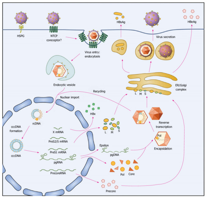
Recently, researchers have become interested in modelling, monitoring, and treatment of hepatitis B virus infection. Understanding the various connections between pathogens, immune systems, and general liver function is crucial. In this study, we propose a higher-order stochastically modified delay differential model for the evolution of hepatitis B virus transmission involving defensive cells. Taking into account environmental stimuli and ambiguities, we presented numerical solutions of the fractal-fractional hepatitis B virus model based on the exponential decay kernel that reviewed the hepatitis B virus immune system involving cytotoxic T lymphocyte immunological mechanisms. Furthermore, qualitative aspects of the system are analyzed such as the existence-uniqueness of the non-negative solution, where the infection endures stochastically as a result of the solution evolving within the predetermined system's equilibrium state. In certain settings, infection-free can be determined, where the illness settles down tremendously with unit probability. To predict the viability of the fractal-fractional derivative outcomes, a novel numerical approach is used, resulting in several remarkable modelling results, including a change in fractional-order $\delta$ with constant fractal-dimension $\varpi$ , $\delta$ with changing $\varpi$ , and $\delta$ with changing both $\delta$ and $\varpi$ . White noise concentration has a significant impact on how bacterial infections are treated.

Keywords:

HBV model,
Fractal-fractional Caputo-Fabrizio differential operators,
existence and uniqueness,
qualitative analysis,
numerical solution

Citation: Maysaa Al Qurashi, Saima Rashid, Fahd Jarad. A computational study of a stochastic fractal-fractional hepatitis B virus infection incorporating delayed immune reactions via the exponential decay[J]. Mathematical Biosciences and Engineering, 2022, 19(12): 12950-12980. doi: 10.3934/mbe.2022605

Related Papers:

[1]	Quanguo Chen, Yong Deng . Hopf algebra structures on generalized quaternion algebras. Electronic Research Archive, 2024, 32(5): 3334-3362. doi: 10.3934/era.2024154
[2]	Kengo Matsumoto . $C^$ -algebras associated with asymptotic equivalence relations defined by hyperbolic toral automorphisms. Electronic Research Archive, 2021, 29(4): 2645-2656. doi: 10.3934/era.2021006*
[3]	Peigen Cao, Fang Li, Siyang Liu, Jie Pan . A conjecture on cluster automorphisms of cluster algebras. Electronic Research Archive, 2019, 27(0): 1-6. doi: 10.3934/era.2019006
[4]	Dong Su, Shilin Yang . Representation rings of extensions of Hopf algebra of Kac-Paljutkin type. Electronic Research Archive, 2024, 32(9): 5201-5230. doi: 10.3934/era.2024240
[5]	Hongyan Guo . Automorphism group and twisted modules of the twisted Heisenberg-Virasoro vertex operator algebra. Electronic Research Archive, 2021, 29(4): 2673-2685. doi: 10.3934/era.2021008
[6]	Bing Sun, Liangyun Chen, Yan Cao . On the universal $\alpha$ -central extensions of the semi-direct product of Hom-preLie algebras. Electronic Research Archive, 2021, 29(4): 2619-2636. doi: 10.3934/era.2021004
[7]	Neşet Deniz Turgay . On the mod p Steenrod algebra and the Leibniz-Hopf algebra. Electronic Research Archive, 2020, 28(2): 951-959. doi: 10.3934/era.2020050
[8]	Jingjing Hai, Xian Ling . Normalizer property of finite groups with almost simple subgroups. Electronic Research Archive, 2022, 30(11): 4232-4237. doi: 10.3934/era.2022215
[9]	Xue Yu . Orientable vertex imprimitive complete maps. Electronic Research Archive, 2024, 32(4): 2466-2477. doi: 10.3934/era.2024113
[10]	Hongliang Chang, Yin Chen, Runxuan Zhang . A generalization on derivations of Lie algebras. Electronic Research Archive, 2021, 29(3): 2457-2473. doi: 10.3934/era.2020124

Abstract

1. Introduction

The study of algebraic automorphisms on different algebraic systems is a classic direction in algebra. Usually, it is very difficult to determine the automorphisms of an algebra. How to describe the automorphisms in an algebra is still an open problem. A well-studied example is the automorphism group of an incidence algebra ^[1,2]. Andruskiewitsch and Dumas studied the algebra automorphisms and Hopf algebra automorphisms of the positive part of the quantum enveloping algebra of simple complex finite-dimensional Lie algebras in ^[3]. For more works on the algebra automorphisms of other algebras, please refer to ^{[4,5,6,7,8,9,10]}.

The purpose of this paper is to find an effective method to determine the automorphisms of finite-dimensional algebras. Using the method, we not only describe all automorphisms of low-dimensional algebras, but also identify some good automorphisms of high-dimensional algebras.

The paper is organized as follows:

In Section 2, we establish a criterion for automorphisms of finite-dimensional algebras. In Section 3, as an application, we give all automorphisms of the single-parameter generalized quaternion algebra. As special cases of the single-parameter generalized quaternion algebra, all automorphisms on the semi-quaternion algebra and the split semi-quaternion algebra are given. Since Sweedler's 4-dimensional Hopf algebra, as an algebra, is a split semi-quaternion algebra, all algebraic automorphisms in Sweedler's 4-dimensional Hopf algebra are described.

2. The criteria for automorphisms on finite-dimensional algebras

Throughout the paper, $\mathbb{R}$ denotes the real number field. All algebras are over $\mathbb{R}$ , and linear refers to $\mathbb{R}$ -linear. Given a matrix $M$ , $M^{T}$ denotes the transpose of $M$ .

Let

$\eta_{1} = \left( \begin{array}{c} 1\\ 0 \\ \vdots \\ 0\\ \end{array} \right),\eta_{2} = \left( \begin{array}{c} 0\\ 1 \\ \vdots \\ 0\\ \end{array} \right),\cdots, \eta_{n} = \left( \begin{array}{c} 0\\ 0 \\ \vdots \\ 1\\ \end{array} \right)$

be the standard basis of $\mathbb{R}^{n}$ .

Let $A$ be a finite-dimensional algebra with unit $1$ and generators $g_{1}, g_{2}, \cdots, g_{s}$ which are subject to certain relationships. Assume that $\{\alpha_{1} = 1, \alpha_{2}, \cdots, \alpha_{n}\}$ is a basis for $A$ . Using the relationships among the $g_{i}$ , we have

$\begin{equation} \left( \begin{array}{c} \alpha_{1}\\ \alpha_{2} \\ \vdots \\ \alpha_{n}\\ \end{array} \right)(\alpha_{1},\alpha_{2},\cdots, \alpha_{n}) = \mathbf{U}_{1}\alpha_{1}+\mathbf{U}_{2}\alpha_{2}+\cdots+\mathbf{U}_{n}\alpha_{n}, \end{equation}$

(2.1)

where each $\mathbf{U_{i}}$ is a $n\times n$ digital matrix. By dividing $\mathbf{U}_{i}$ into block matrices by the columns, we obtain

$\mathbf{U}_{i} = (_{i}\gamma_{1},_{i}\gamma_{2},\cdots, _{i}\gamma_{n}), \ _{i}\gamma_{j} = \left( \begin{array}{c} _{i}u_{1j} \\ _{i}u_{2j} \\ \vdots \\ _{i}u_{nj} \\ \end{array} \right).$

Construct the following matrices

$\mathbf{W}_{i} = (_{1}\gamma_{i}, _{2}\gamma_{i}, \cdots, _{n}\gamma_{i}), i = 1,2,\cdots, n.$

Definition 2.1. With the matrices $\mathbf{U}_{i}(i = 1, 2, \cdots, n)$ as above. We call $\mathbf{W}_{i}(i = 1, 2, \cdots, n)$ the matrix induced from the $i$ -th columns of $\{U_{j}\}_{j = 1}^{n}$ .

Lemma 2.2. Let $\mathcal{P}$ be a linear transformation on $A$ , and

$P = \left( \begin{array}{cccc} a_{11} & a_{12}& \cdots & a_{1n}\\ a_{21} & a_{22}& \cdots & a_{2n} \\ \vdots &\vdots& \vdots & \vdots \\ a_{n1} & a_{n2}& \cdots & a_{nn} \\ \end{array} \right) = (\xi_{1},\xi_{2},\cdots,\xi_{n}),$

the matrix of $\mathcal{P}$ with respect to the basis $\alpha_{1}, \alpha_{2}, \cdots, \alpha_{n}$ . Then we have

$\begin{eqnarray} \mathcal{P}(\alpha_{i})\mathcal{P}(\alpha_{j}) = (\alpha_{1}, \alpha_{2},\cdots, \alpha_{n})\left( \begin{array}{cccc} \xi_{j}& & & \\ & \xi_{j} & & \\ & & \ddots& \\ & & &\xi_{j}\\ \end{array} \right)^{T}\mathbf{C}^{T}\xi_{i}, \end{eqnarray}$

(2.2)

for all $i, j = 1, 2, \cdots, n$ , where

$\mathbf{C} = (\mathbf{U}_{1}, \mathbf{U}_{2}, \cdots , \mathbf{U}_{n}).$

Proof. For all $i, j$ , since

$\begin{eqnarray*} \mathcal{P}(\alpha_{i})\mathcal{P}(\alpha_{j}) & = &\xi_{i}^{T} \left( \begin{array}{c} \alpha_{1} \\ \alpha_{2} \\ \vdots \\ \alpha_{n} \\ \end{array} \right) (\alpha_{1},\alpha_{2},\cdots, \alpha_{n})\xi_{j}\\ & = &\xi_{i}^{T} \left( \mathbf{U}_{1}\alpha_{1}+\mathbf{U}_{2}\alpha_{2}+\cdots+\mathbf{U}_{n}\alpha_{n} \right)\xi_{j}\\ & = &\xi_{i}^{T} \mathbf{U}_{1} \xi_{j}\alpha_{1} +\xi_{i}^{T} \mathbf{U}_{2}\xi_{j}\alpha_{2}+\cdots +\xi_{i}^{T} \mathbf{U}_{n} \xi_{j}\alpha_{n}\\ & = &\xi_{i} ^{T}\mathbf{C}\left( \begin{array}{cccc} \xi_{j}& & & \\ & \xi_{j} & & \\ & & \ddots& \\ & & &\xi_{j}\\ \end{array} \right) \left( \begin{array}{c} \alpha_{1} \\ \alpha_{2} \\ \vdots \\ \alpha_{n} \\ \end{array} \right), \end{eqnarray*}$

it follows that (2.2) holds. □

Example 2.3. Recall that a single-parameter quaternion $q$ is an expression of the form

$q = a_{0}+a_{1}e_{1}+a_{2}e_{2}+a_{3}e_{3},$

where $a_{0}, a_{1}, a_{2}, a_{3}$ are real numbers and $e_{1}, e_{2}, e_{3}$ satisfy the following equalities:

$e_{1}^{2} = -\mu, e_{2}^{2} = 0, e_{3}^{2} = 0, e_{1}e_{2} = e_{3} = -e_{2}e_{1}, e_{2}e_{3} = 0 = -e_{3}e_{2}, e_{3}e_{1} = \mu e_{2} = -e_{1}e_{3},$

where $0\neq\mu\in \mathbb{R}$ . The set of single-parameter quaternions is denoted by $\mathbb{H}_{\mu}$ ^[8], and $\mathbb{H}_{\mu}$ is an associative algebra. We call $\mathbb{H}_{\mu}$ an algebra of single-parameter quaternions (or single-parameter quaternion algebra).

Observe that $\mathbb{H}_{\mu}$ is a 4-dimensional algebra with basis $1, e_{1}, e_{2}, e_{3}$ . By computing

$\begin{eqnarray*} \left( \begin{array}{c} 1\\ e_{1} \\ e_{2} \\ e_{3}\\ \end{array} \right)(1,e_{1},e_{2}, e_{3})& = & \left( \begin{array}{cccc} 1 & e_{1}& e_{2} & e_{3} \\ e_{1} &-\mu & e_{3} & -\mu e_{2}\\ e_{2} & -e_{3} & 0 & 0\\ e_{3} & \mu e_{2} & 0 & 0 \\ \end{array} \right)\\ & = & \left( \begin{array}{cccc} 1 & 0& 0 & 0 \\ 0 & -\mu & 0 & 0\\ 0 &0& 0 & 0\\ 0 & 0 & 0 & 0 \\ \end{array} \right)1+\left( \begin{array}{cccc} 0 & 1 & 0 & 0 \\ 1 & 0 & 0 & 0 \\ 0 & 0 & 0 & 0 \\ 0 & 0 & 0 & 0 \\ \end{array} \right)e_{1}\\ &&+\left( \begin{array}{cccc} 0 & 0 & 1 & 0 \\ 0 & 0 & 0 & -\mu \\ 1 & 0 & 0 & 0 \\ 0 & \mu & 0 & 0 \\ \end{array} \right)e_{2}+\left( \begin{array}{cccc} 0 & 0 & 0 & 1 \\ 0 & 0 & 1 & 0 \\ 0 & -1 & 0 & 0 \\ 1 & 0 & 0 & 0 \\ \end{array} \right)e_{3}. \end{eqnarray*}$

We have the corresponding $\mathbf{U}_{i} (i = 1, 2, 3, 4)$ as follows:

$\mathbf{U}_{1} = \left( \begin{array}{cccc} 1 & 0 & 0 & 0 \\ 0 & -\mu & 0 & 0 \\ 0 & 0 & 0 & 0 \\ 0 & 0 & 0 & 0 \\ \end{array} \right), \mathbf{U}_{2} = \left( \begin{array}{cccc} 0 & 1 & 0 & 0 \\ 1 & 0 & 0 & 0 \\ 0 & 0 & 0 & 0 \\ 0 & 0 & 0 & 0 \\ \end{array} \right),\mathbf{U}_{3} = \left( \begin{array}{cccc} 0 & 0 & 1 & 0 \\ 0 & 0 & 0 & -\mu \\ 1 & 0 & 0 & 0 \\ 0 & \mu & 0 & 0 \\ \end{array} \right),$

$\mathbf{U}_{4} = \left( \begin{array}{cccc} 0 & 0 & 0 & 1 \\ 0 & 0 & 1 & 0 \\ 0 & -1 & 0 & 0 \\ 1 & 0 & 0 & 0 \\ \end{array} \right).$

Thus we have

$\mathbf{C} = \left( \begin{array}{cccccccccccccccc} 1 & 0 & 0 & 0 & 0 & 1 & 0 & 0 & 0 & 0 & 1 & 0 & 0 & 0 & 0 & 1 \\ 0 & -\mu & 0 & 0 & 1 & 0 & 0 & 0 & 0 & 0 & 0 & -\mu & 0 & 0 & 1 & 0 \\ 0 & 0 & 0 & 0 & 0 & 0 & 0 & 0 & 1 & 0 & 0 & 0 & 0 & -1 & 0 & 0 \\ 0 & 0 & 0 & 0 & 0 & 0 & 0 & 0 & 0 & \mu & 0 & 0 & 1 & 0 & 0 & 0 \\ \end{array} \right).$

Let $\mathcal{P}$ be a linear transformation on $\mathbb{H}_{\mu}$ , and

$P = \left( \begin{array}{cccc} a_{11} & a_{12}& a_{13} & a_{14}\\ a_{21} & a_{22}& a_{23} & a_{24} \\ a_{31} & a_{32}& a_{33} & a_{34} \\ a_{41} & a_{42}& a_{43} & a_{44} \\ \end{array} \right) = (\xi_{1},\xi_{2},\xi_{3},\xi_{4}),$

the matrix of $\mathcal{P}$ with respect to the basis $\alpha_{1} = 1, \alpha_{2} = e_{1}, \alpha_{3} = e_{2}, \alpha_{4} = e_{3}$ . For instance, we aim to compute $\mathcal{P}(e_{1})\mathcal{P}(e_{2})$ , i.e., $\mathcal{P}(\alpha_{2})\mathcal{P}(\alpha_{3})$ . Since

$\left( \begin{array}{cccc} a_{13} & 0 & 0 & 0 \\ a_{23} & 0 & 0 & 0 \\ a_{33} & 0 & 0 & 0 \\ a_{43} & 0 & 0 & 0 \\ 0 & a_{13} & 0 & 0 \\ 0 & a_{23} & 0 & 0 \\ 0 & a_{33} & 0 & 0 \\ 0 & a_{43} & 0 & 0 \\ 0 & 0 & a_{13} & 0 \\ 0 & 0 & a_{23} & 0 \\ 0 & 0 & a_{33} & 0 \\ 0 & 0 & a_{43} & 0 \\ 0 & 0 & 0 & a_{13} \\ 0 & 0 & 0 & a_{23} \\ 0 & 0 & 0 & a_{33} \\ 0 & 0 & 0 & a_{43} \\ \end{array} \right)^{T}\mathbf{C}^{T}\left( \begin{array}{c} a_{12} \\ a_{22} \\ a_{32} \\ a_{42} \\ \end{array} \right) = \left( \begin{array}{c} a_{12} a_{13}-a_{22} a_{23} \mu \\ a_{13} a_{22}+a_{12} a_{23} \\ -a_{22} a_{43} \mu +a_{23} a_{42} \mu +a_{13} a_{32}+a_{12} a_{33} \\ -a_{23} a_{32}+a_{22} a_{33}+a_{13} a_{42}+a_{12} a_{43} \\ \end{array} \right)$

by Lemma 2.2, we have

$\mathcal{P}(e_{1})\mathcal{P}(e_{2}) = (1,e_{1},e_{2},e_{3})\left( \begin{array}{c} a_{12} a_{13}-a_{22} a_{23} \mu \\ a_{13} a_{22}+a_{12} a_{23} \\ -a_{22} a_{43} \mu +a_{23} a_{42} \mu +a_{13} a_{32}+a_{12} a_{33} \\ -a_{23} a_{32}+a_{22} a_{33}+a_{13} a_{42}+a_{12} a_{43} \\ \end{array} \right).$

Theorem 2.4. With notation as shown in Lemma 2.2. Then $\mathcal{P}$ is an automorphism if and only if $\xi_{1} = \eta_{1}$ and the matrix $P$ is an invertible matrix and satisfies the following equation:

$\begin{equation} (\mathbf{W}_{1},\mathbf{W}_{2},\cdots, \mathbf{W}_{n})\left( \begin{array}{cccc} P & 0 &0 & 0 \\ 0 & P & 0 & 0 \\ 0 & 0 & \ddots& 0 \\ 0 & 0 & 0 & P \\ \end{array} \right)^{T} = P^{T}\mathbf{C}\left( \begin{array}{cccc} P & 0 &0 & 0 \\ 0 & P & 0 & 0 \\ 0 & 0 & \ddots& 0 \\ 0 & 0 & 0 & P \\ \end{array} \right)\mathbf{K}, \end{equation}$

(2.3)

where $\mathbf{C}$ is shown in Lemma 2.2 and

$\mathbf{K} = \left( \begin{array}{ccccccccccccc} \eta_1 & 0 & \cdots & 0 & \eta_2 & 0 & \cdots & 0 & \cdots & \eta_n & 0 & \cdots & 0 \\ 0 & \eta_1 & \cdots & 0 & 0 & \eta_2 & \cdots & 0 & \cdots & 0 & \eta_n & \cdots & 0 \\ \vdots & \vdots & \ddots & \vdots & \vdots & \vdots & \ddots & \vdots & \cdots & \vdots & \vdots & \ddots & \vdots \\ 0 & 0 & \cdots & \eta_1 & 0 & 0 & \cdots & \eta_2 & \cdots & 0 & 0 & \cdots & \eta_n \\ \end{array} \right).$

Proof. From (2.1), it follows that

$\begin{equation} \alpha_{i} \alpha_{j} = (\alpha_{1}, \alpha_{2}, \cdots, \alpha_{n})\left( \begin{array}{c} _{1}u_{ij} \\ _{2}u_{ij} \\ \vdots \\ _{n}u_{ij} \\ \end{array} \right), \forall i,j = 1,2,\cdots, n. \end{equation}$

(2.4)

For a fixed $j$ , by using (2.4), we have

$\mathcal{P}(\alpha_{i}\alpha_{j}) = (\alpha_{1},\alpha_{2},\cdots,\alpha_{n})P\left( \begin{array}{c} _{1}u_{ij} \\ _{2}u_{ij} \\ \vdots \\ _{n}u_{ij} \\ \end{array} \right).$

Since $\mathcal{P}(\alpha_{i}\alpha_{j}) = \mathcal{P}(\alpha_{i})\mathcal{P}(\alpha_{j})$ , for all $i$ , it follows that

$\left( \begin{array}{cccc} \xi_{j}& & & \\ & \xi_{j} & & \\ & & \ddots& \\ & & &\xi_{j}\\ \end{array} \right)^{T}\mathbf{C}^{T}\xi_{i} = P\left( \begin{array}{c} _{1}u_{ij} \\ _{2}u_{ij} \\ \vdots \\ _{n}u_{ij} \\ \end{array} \right),$

which is equivalent to

$\begin{eqnarray*} \left( \begin{array}{cccc} \xi_{j}& & & \\ & \xi_{j} & & \\ & & \ddots& \\ & & &\xi_{j}\\ \end{array} \right)^{T}\mathbf{C}^{T}P = P \left( \begin{array}{cccc} _{1}u_{1j} & _{1}u_{2j} & \cdots & _{1}u_{nj} \\ _{2}u_{1j}& _{2}u_{2j} & \cdots & _{2}u_{nj} \\ \vdots & \vdots &\vdots & \vdots \\ _{n}u_{1j} & _{n}u_{2j} & \cdots & _{n}u_{nj} \\ \end{array} \right) = P \mathbf{W}^{T}_{j}. \end{eqnarray*}$

Thus

$\begin{eqnarray*} &&(\mathbf{W}_{1},\mathbf{W}_{2},\cdots, \mathbf{W}_{n})\left( \begin{array}{cccc} P & 0 &0 & 0 \\ 0 & P & 0 & 0 \\ 0 & 0 & \ddots& 0 \\ 0 & 0 & 0 & P \\ \end{array} \right)^{T}\\ & = &P^{T}\mathbf{C}\left( \begin{array}{ccccccccccccc} \xi_{1} & 0 & \cdots & 0 & \xi_{2} & 0 & \cdots & 0 & \cdots & \xi_{n} & 0 & \cdots & 0 \\ 0 & \xi_{1} & \cdots & 0 & 0 & \xi_{2} & \cdots & 0 & \cdots & 0 & \xi_{n} & \cdots & 0 \\ \vdots & \vdots & \ddots & \vdots & \vdots & \vdots & \ddots & \vdots & \cdots & \vdots & \vdots & \ddots & \vdots \\ 0 & 0 & \cdots & \xi_{1} & 0 & 0 & \cdots & \xi_{2} & \cdots & 0 & 0 & \cdots & \xi_{n} \\ \end{array} \right)\\ & = &P^{T}\mathbf{C}\left( \begin{array}{cccc} P & 0 &0 & 0 \\ 0 & P & 0 & 0 \\ 0 & 0 & \ddots& 0 \\ 0 & 0 & 0 & P \\ \end{array} \right)\mathbf{K}. \end{eqnarray*}$

From $\mathcal{P}(1) = 1$ , we obtain $\xi_{1} = \eta_{1}$ . The proof is completed.

Example 2.5. Let $\mathbf{U}_{i} (i = 1, 2, 3, 4)$ and $\mathbf{C}$ be given in Example 2.3. By Definition 2.1, we can obtain the desired $\mathbf{W}_{i}(i = 1, 2, 3, 4)$ as follows:

$\mathbf{W}_{1} = \left( \begin{array}{cccc} 1 & 0 & 0 & 0 \\ 0 & 1 & 0 & 0 \\ 0 & 0 & 1 & 0 \\ 0 & 0 & 0 & 1 \\ \end{array} \right), \mathbf{W}_{2} = \left( \begin{array}{cccc} 0 & 1 & 0 & 0 \\ -\mu & 0 & 0 & 0 \\ 0 & 0 & 0 & -1 \\ 0 & 0 & \mu & 0 \\ \end{array} \right), \mathbf{W}_{3} = \left( \begin{array}{cccc} 0 & 0 & 1 & 0 \\ 0 & 0 & 0 & 1 \\ 0 & 0 & 0 & 0 \\ 0 & 0 & 0 & 0 \\ \end{array} \right),$

$\mathbf{W}_{4} = \left( \begin{array}{cccc} 0 & 0 & 0 & 1 \\ 0 & 0 & -\mu & 0 \\ 0 & 0 & 0 & 0 \\ 0 & 0 & 0 & 0 \\ \end{array} \right).$

Thus, we have

$(\mathbf{W}_{1},\mathbf{W}_{2},\mathbf{W}_{3},\mathbf{W}_{4}) = \left( \begin{array}{cccccccccccccccc} 1 & 0 & 0 & 0 & 0 & 1 & 0 & 0 & 0 & 0 & 1 & 0 & 0 & 0 & 0 & 1 \\ 0 & 1 & 0 & 0 & -\mu & 0 & 0 & 0 & 0 & 0 & 0 & 1 & 0 & 0 & -\mu & 0 \\ 0 & 0 & 1 & 0 & 0 & 0 & 0 & -1 & 0 & 0 & 0 & 0 & 0 & 0 & 0 & 0 \\ 0 & 0 & 0 & 1 & 0 & 0 & \mu & 0 & 0 & 0 & 0 & 0 & 0 & 0 & 0 & 0 \\ \end{array} \right)$

and

$\mathbf{K} = \left( \begin{array}{cccccccccccccccc} 1 & 0 & 0 & 0 & 0 & 0 & 0 & 0 & 0 & 0 & 0 & 0 & 0 & 0 & 0 & 0 \\ 0 & 0 & 0 & 0 & 1 & 0 & 0 & 0 & 0 & 0 & 0 & 0 & 0 & 0 & 0 & 0 \\ 0 & 0 & 0 & 0 & 0 & 0 & 0 & 0 & 1 & 0 & 0 & 0 & 0 & 0 & 0 & 0 \\ 0 & 0 & 0 & 0 & 0 & 0 & 0 & 0 & 0 & 0 & 0 & 0 & 1 & 0 & 0 & 0 \\ 0 & 1 & 0 & 0 & 0 & 0 & 0 & 0 & 0 & 0 & 0 & 0 & 0 & 0 & 0 & 0 \\ 0 & 0 & 0 & 0 & 0 & 1 & 0 & 0 & 0 & 0 & 0 & 0 & 0 & 0 & 0 & 0 \\ 0 & 0 & 0 & 0 & 0 & 0 & 0 & 0 & 0 & 1 & 0 & 0 & 0 & 0 & 0 & 0 \\ 0 & 0 & 0 & 0 & 0 & 0 & 0 & 0 & 0 & 0 & 0 & 0 & 0 & 1 & 0 & 0 \\ 0 & 0 & 1 & 0 & 0 & 0 & 0 & 0 & 0 & 0 & 0 & 0 & 0 & 0 & 0 & 0 \\ 0 & 0 & 0 & 0 & 0 & 0 & 1 & 0 & 0 & 0 & 0 & 0 & 0 & 0 & 0 & 0 \\ 0 & 0 & 0 & 0 & 0 & 0 & 0 & 0 & 0 & 0 & 1 & 0 & 0 & 0 & 0 & 0 \\ 0 & 0 & 0 & 0 & 0 & 0 & 0 & 0 & 0 & 0 & 0 & 0 & 0 & 0 & 1 & 0 \\ 0 & 0 & 0 & 1 & 0 & 0 & 0 & 0 & 0 & 0 & 0 & 0 & 0 & 0 & 0 & 0 \\ 0 & 0 & 0 & 0 & 0 & 0 & 0 & 1 & 0 & 0 & 0 & 0 & 0 & 0 & 0 & 0 \\ 0 & 0 & 0 & 0 & 0 & 0 & 0 & 0 & 0 & 0 & 0 & 1 & 0 & 0 & 0 & 0 \\ 0 & 0 & 0 & 0 & 0 & 0 & 0 & 0 & 0 & 0 & 0 & 0 & 0 & 0 & 0 & 1 \\ \end{array} \right).$

3. Application to $\mathbb{H}_{\mu}$

In this section, we consider the application of Theorem 2.4 to $\mathbb{H}_{\mu}$ . To describe all automorphisms on $\mathbb{H}_{\mu}$ , we need to determine the matrices $P$ that satisfy the condition (2.3). Let

$P = \left( \begin{array}{cccc} 1 & a_{12} & a_{13} & a_{14} \\ 0 & a_{22} & a_{23} & a_{24} \\ 0 & a_{32} & a_{33} & a_{34} \\ 0 & a_{42} & a_{43} & a_{44} \\ \end{array} \right).$

Since

$\begin{eqnarray*} &&\text{LHS of (2.3)} \\& = & (\mathbf{W}_{1},\mathbf{W}_{2},\mathbf{W}_{3}, \mathbf{W}_{4})\left( \begin{array}{cccc} P & 0 &0 & 0 \\ 0 & P & 0 & 0 \\ 0 & 0 & P& 0 \\ 0 & 0 & 0 & P \\ \end{array} \right)^{T}\\ & = &\left( \begin{array}{cccccccccccccccc} 1 & 0 & 0 & 0 & 0 & 1 & 0 & 0 & 0 & 0 & 1 & 0 & 0 & 0 & 0 & 1 \\ 0 & 1 & 0 & 0 & -\mu & 0 & 0 & 0 & 0 & 0 & 0 & 1 & 0 & 0 & -\mu & 0 \\ 0 & 0 & 1 & 0 & 0 & 0 & 0 & -1 & 0 & 0 & 0 & 0 & 0 & 0 & 0 & 0 \\ 0 & 0 & 0 & 1 & 0 & 0 & \mu & 0 & 0 & 0 & 0 & 0 & 0 & 0 & 0 & 0 \\ \end{array} \right)\\ &&\left( \begin{array}{cccccccccccccccc} 1 & a_{12} & a_{13} & a_{14} & 0 & 0 & 0 & 0 & 0 & 0 & 0 & 0 & 0 & 0 & 0 & 0 \\ 0 & a_{22} & a_{23} & a_{24} & 0 & 0 & 0 & 0 & 0 & 0 & 0 & 0 & 0 & 0 & 0 & 0 \\ 0 & a_{32} & a_{33} & a_{34} & 0 & 0 & 0 & 0 & 0 & 0 & 0 & 0 & 0 & 0 & 0 & 0 \\ 0 & a_{42} & a_{43} & a_{44} & 0 & 0 & 0 & 0 & 0 & 0 & 0 & 0 & 0 & 0 & 0 & 0 \\ 0 & 0 & 0 & 0 & 1 & a_{12} & a_{13} & a_{14} & 0 & 0 & 0 & 0 & 0 & 0 & 0 & 0 \\ 0 & 0 & 0 & 0 & 0 & a_{22} & a_{23} & a_{24} & 0 & 0 & 0 & 0 & 0 & 0 & 0 & 0 \\ 0 & 0 & 0 & 0 & 0 & a_{32} & a_{33} & a_{34} & 0 & 0 & 0 & 0 & 0 & 0 & 0 & 0 \\ 0 & 0 & 0 & 0 & 0 & a_{42} & a_{43} & a_{44} & 0 & 0 & 0 & 0 & 0 & 0 & 0 & 0 \\ 0 & 0 & 0 & 0 & 0 & 0 & 0 & 0 & 1 & a_{12} & a_{13} & a_{14} & 0 & 0 & 0 & 0 \\ 0 & 0 & 0 & 0 & 0 & 0 & 0 & 0 & 0 & a_{22} & a_{23} & a_{24} & 0 & 0 & 0 & 0 \\ 0 & 0 & 0 & 0 & 0 & 0 & 0 & 0 & 0 & a_{32} & a_{33} & a_{34} & 0 & 0 & 0 & 0 \\ 0 & 0 & 0 & 0 & 0 & 0 & 0 & 0 & 0 & a_{42} & a_{43} & a_{44} & 0 & 0 & 0 & 0 \\ 0 & 0 & 0 & 0 & 0 & 0 & 0 & 0 & 0 & 0 & 0 & 0 & 1 & a_{12} & a_{13} & a_{14} \\ 0 & 0 & 0 & 0 & 0 & 0 & 0 & 0 & 0 & 0 & 0 & 0 & 0 & a_{22} & a_{23} & a_{24} \\ 0 & 0 & 0 & 0 & 0 & 0 & 0 & 0 & 0 & 0 & 0 & 0 & 0 & a_{32} & a_{33} & a_{34} \\ 0 & 0 & 0 & 0 & 0 & 0 & 0 & 0 & 0 & 0 & 0 & 0 & 0 & a_{42} & a_{43} & a_{44} \\ \end{array} \right)^{T}\\ & = &(\mathbf{M}_{1}, \mathbf{M}_{2},\mathbf{M}_{3},\mathbf{M}_{4}), \end{eqnarray*}$

where

$\mathbf{M}_{1} = \left( \begin{array}{cccc} 1 & 0 & 0 & 0 \\ a_{12} & a_{22} & a_{32} & a_{42} \\ a_{13} & a_{23} & a_{33} & a_{43} \\ a_{14} & a_{24} & a_{34} & a_{44} \\ \end{array} \right), \mathbf{M}_{2} = \left( \begin{array}{cccc} a_{12} & a_{22} & a_{32} & a_{42} \\ -\mu & 0 & 0 & 0 \\ -a_{14} & -a_{24} & -a_{34} & -a_{44} \\ a_{13} \mu & a_{23} \mu & a_{33} \mu & a_{43} \mu \\ \end{array} \right),$

$\mathbf{M}_{3} = \left( \begin{array}{cccc} a_{13} & a_{23} & a_{33} & a_{43} \\ a_{14} & a_{24} & a_{34} & a_{44} \\ 0 & 0 & 0 & 0 \\ 0 & 0 & 0 & 0 \\ \end{array} \right), \mathbf{M}_{4} = \left( \begin{array}{cccc} a_{14} & a_{24} & a_{34} & a_{44} \\ a_{13} (-\mu ) & a_{23} (-\mu ) & a_{33} (-\mu ) & a_{43} (-\mu ) \\ 0 & 0 & 0 & 0 \\ 0 & 0 & 0 & 0 \\ \end{array} \right),$

and

$\begin{eqnarray*} &&\text{RHS of (2.3)} \\& = & P^{T}\mathbf{C}\left( \begin{array}{cccc} P & 0 &0 & 0 \\ 0 & P & 0 & 0 \\ 0 & 0 & \ddots& 0 \\ 0 & 0 & 0 & P \\ \end{array} \right)\mathbf{K}\\ & = &\left( \begin{array}{cccc} 1 & a_{12} & a_{13} & a_{14} \\ 0 & a_{22} & a_{23} & a_{24} \\ 0 & a_{32} & a_{33} & a_{34} \\ 0 & a_{42} & a_{43} & a_{44} \\ \end{array} \right)^{T}\left( \begin{array}{cccccccccccccccc} 1 & 0 & 0 & 0 & 0 & 1 & 0 & 0 & 0 & 0 & 1 & 0 & 0 & 0 & 0 & 1 \\ 0 & -\mu & 0 & 0 & 1 & 0 & 0 & 0 & 0 & 0 & 0 & -\mu & 0 & 0 & 1 & 0 \\ 0 & 0 & 0 & 0 & 0 & 0 & 0 & 0 & 0 & 1 & 0 & 0 & 0 & -1 & 0 & 0 \\ 0 & 0 & 0 & 0 & 0 & 0 & 0 & 0 & 0 & 0 & \mu & 0 & 1 & 0 & 0 & 0 \\ \end{array} \right)\\ &&\left( \begin{array}{cccccccccccccccc} 1 & a_{12} & a_{13} & a_{14} & 0 & 0 & 0 & 0 & 0 & 0 & 0 & 0 & 0 & 0 & 0 & 0 \\ 0 & a_{22} & a_{23} & a_{24} & 0 & 0 & 0 & 0 & 0 & 0 & 0 & 0 & 0 & 0 & 0 & 0 \\ 0 & a_{32} & a_{33} & a_{34} & 0 & 0 & 0 & 0 & 0 & 0 & 0 & 0 & 0 & 0 & 0 & 0 \\ 0 & a_{42} & a_{43} & a_{44} & 0 & 0 & 0 & 0 & 0 & 0 & 0 & 0 & 0 & 0 & 0 & 0 \\ 0 & 0 & 0 & 0 & 1 & a_{12} & a_{13} & a_{14} & 0 & 0 & 0 & 0 & 0 & 0 & 0 & 0 \\ 0 & 0 & 0 & 0 & 0 & a_{22} & a_{23} & a_{24} & 0 & 0 & 0 & 0 & 0 & 0 & 0 & 0 \\ 0 & 0 & 0 & 0 & 0 & a_{32} & a_{33} & a_{34} & 0 & 0 & 0 & 0 & 0 & 0 & 0 & 0 \\ 0 & 0 & 0 & 0 & 0 & a_{42} & a_{43} & a_{44} & 0 & 0 & 0 & 0 & 0 & 0 & 0 & 0 \\ 0 & 0 & 0 & 0 & 0 & 0 & 0 & 0 & 1 & a_{12} & a_{13} & a_{14} & 0 & 0 & 0 & 0 \\ 0 & 0 & 0 & 0 & 0 & 0 & 0 & 0 & 0 & a_{22} & a_{23} & a_{24} & 0 & 0 & 0 & 0 \\ 0 & 0 & 0 & 0 & 0 & 0 & 0 & 0 & 0 & a_{32} & a_{33} & a_{34} & 0 & 0 & 0 & 0 \\ 0 & 0 & 0 & 0 & 0 & 0 & 0 & 0 & 0 & a_{42} & a_{43} & a_{44} & 0 & 0 & 0 & 0 \\ 0 & 0 & 0 & 0 & 0 & 0 & 0 & 0 & 0 & 0 & 0 & 0 & 1 & a_{12} & a_{13} & a_{14} \\ 0 & 0 & 0 & 0 & 0 & 0 & 0 & 0 & 0 & 0 & 0 & 0 & 0 & a_{22} & a_{23} & a_{24} \\ 0 & 0 & 0 & 0 & 0 & 0 & 0 & 0 & 0 & 0 & 0 & 0 & 0 & a_{32} & a_{33} & a_{34} \\ 0 & 0 & 0 & 0 & 0 & 0 & 0 & 0 & 0 & 0 & 0 & 0 & 0 & a_{42} & a_{43} & a_{44} \\ \end{array} \right)\\ &&\left( \begin{array}{cccccccccccccccc} 1 & 0 & 0 & 0 & 0 & 0 & 0 & 0 & 0 & 0 & 0 & 0 & 0 & 0 & 0 & 0 \\ 0 & 0 & 0 & 0 & 1 & 0 & 0 & 0 & 0 & 0 & 0 & 0 & 0 & 0 & 0 & 0 \\ 0 & 0 & 0 & 0 & 0 & 0 & 0 & 0 & 1 & 0 & 0 & 0 & 0 & 0 & 0 & 0 \\ 0 & 0 & 0 & 0 & 0 & 0 & 0 & 0 & 0 & 0 & 0 & 0 & 1 & 0 & 0 & 0 \\ 0 & 1 & 0 & 0 & 0 & 0 & 0 & 0 & 0 & 0 & 0 & 0 & 0 & 0 & 0 & 0 \\ 0 & 0 & 0 & 0 & 0 & 1 & 0 & 0 & 0 & 0 & 0 & 0 & 0 & 0 & 0 & 0 \\ 0 & 0 & 0 & 0 & 0 & 0 & 0 & 0 & 0 & 1 & 0 & 0 & 0 & 0 & 0 & 0 \\ 0 & 0 & 0 & 0 & 0 & 0 & 0 & 0 & 0 & 0 & 0 & 0 & 0 & 1 & 0 & 0 \\ 0 & 0 & 1 & 0 & 0 & 0 & 0 & 0 & 0 & 0 & 0 & 0 & 0 & 0 & 0 & 0 \\ 0 & 0 & 0 & 0 & 0 & 0 & 1 & 0 & 0 & 0 & 0 & 0 & 0 & 0 & 0 & 0 \\ 0 & 0 & 0 & 0 & 0 & 0 & 0 & 0 & 0 & 0 & 1 & 0 & 0 & 0 & 0 & 0 \\ 0 & 0 & 0 & 0 & 0 & 0 & 0 & 0 & 0 & 0 & 0 & 0 & 0 & 0 & 1 & 0 \\ 0 & 0 & 0 & 1 & 0 & 0 & 0 & 0 & 0 & 0 & 0 & 0 & 0 & 0 & 0 & 0 \\ 0 & 0 & 0 & 0 & 0 & 0 & 0 & 1 & 0 & 0 & 0 & 0 & 0 & 0 & 0 & 0 \\ 0 & 0 & 0 & 0 & 0 & 0 & 0 & 0 & 0 & 0 & 0 & 1 & 0 & 0 & 0 & 0 \\ 0 & 0 & 0 & 0 & 0 & 0 & 0 & 0 & 0 & 0 & 0 & 0 & 0 & 0 & 0 & 1 \\ \end{array} \right)\\ & = &(\mathbf{N}_{1}, \mathbf{N}_{2},\mathbf{N}_{3},\mathbf{N}_{4}), \end{eqnarray*}$

where

$\mathbf{N}_{1} = \left( \begin{array}{cccc} 1 & 0 & 0 & 0 \\ a_{12} & a_{22} & a_{32} & a_{42} \\ a_{13} & a_{23} & a_{33} & a_{43} \\ a_{14} & a_{24} & a_{34} & a_{44} \\ \end{array} \right),$

$\mathbf{N}_{2} = \left( \begin{array}{cccc} a_{12} & a_{22} & a_{32} & a_{42} \\ a_{12}^2-a_{22}^2 \mu & 2 a_{12} a_{22} & 2 a_{12} a_{32} & 2 a_{12} a_{42} \\ a_{12} a_{13}-a_{22} a_{23} \mu & a_{13} a_{22}+a_{12} a_{23} & -a_{23} a_{42} \mu +a_{22} a_{43} \mu +a_{13} a_{32}+a_{12} a_{33} & a_{23} a_{32}-a_{22} a_{33}+a_{13} a_{42}+a_{12} a_{43} \\ a_{12} a_{14}-a_{22} a_{24} \mu & a_{14} a_{22}+a_{12} a_{24} & -a_{24} a_{42} \mu +a_{22} a_{44} \mu +a_{14} a_{32}+a_{12} a_{34} & a_{24} a_{32}-a_{22} a_{34}+a_{14} a_{42}+a_{12} a_{44} \\ \end{array} \right) ,$

$\mathbf{N}_{3} = \left( \begin{array}{cccc} a_{13} & a_{23} & a_{33} & a_{43} \\ a_{12} a_{13}-a_{22} a_{23} \mu & a_{13} a_{22}+a_{12} a_{23} & -a_{22} a_{43} \mu +a_{23} a_{42} \mu +a_{13} a_{32}+a_{12} a_{33} & -a_{23} a_{32}+a_{22} a_{33}+a_{13} a_{42}+a_{12} a_{43} \\ a_{13}^2-a_{23}^2 \mu & 2 a_{13} a_{23} & 2 a_{13} a_{33} & 2 a_{13} a_{43} \\ a_{13} a_{14}-a_{23} a_{24} \mu & a_{14} a_{23}+a_{13} a_{24} & -a_{24} a_{43} \mu +a_{23} a_{44} \mu +a_{14} a_{33}+a_{13} a_{34} & a_{24} a_{33}-a_{23} a_{34}+a_{14} a_{43}+a_{13} a_{44} \\ \end{array} \right) ,$

$\mathbf{N}_{4} = \left( \begin{array}{cccc} a_{14} & a_{24} & a_{34} & a_{44} \\ a_{12} a_{14}-a_{22} a_{24} \mu & a_{14} a_{22}+a_{12} a_{24} & -a_{22} a_{44} \mu +a_{24} a_{42} \mu +a_{14} a_{32}+a_{12} a_{34} & -a_{24} a_{32}+a_{22} a_{34}+a_{14} a_{42}+a_{12} a_{44} \\ a_{13} a_{14}-a_{23} a_{24} \mu & a_{14} a_{23}+a_{13} a_{24} & -a_{23} a_{44} \mu +a_{24} a_{43} \mu +a_{14} a_{33}+a_{13} a_{34} & -a_{24} a_{33}+a_{23} a_{34}+a_{14} a_{43}+a_{13} a_{44} \\ a_{14}^2-a_{24}^2 \mu & 2 a_{14} a_{24} & 2 a_{14} a_{34} & 2 a_{14} a_{44} \\ \end{array} \right) ,$

we have $\mathbf{M}_{i} = \mathbf{N}_{i}(i = 1, 2, 3, 4)$ , and obtain the following system of equations:

$a_{22}^2 \mu -a_{12}^2-\mu = 0,$

(a1)

$-2 a_{12} a_{22} = 0,$

(a2)

$-2 a_{12} a_{32} = 0,$

(a3)

$-2 a_{12} a_{42} = 0,$

(a4)

$a_{22} a_{23} \mu -a_{12} a_{13}+a_{14} = 0,$

(a5)

$-a_{13} a_{22}-a_{12} a_{23}+a_{24} = 0,$

(a6)

$-a_{23} a_{42} \mu +a_{22} a_{43} \mu -a_{13} a_{32}-a_{12} a_{33}+a_{34} = 0,$

(a7)

$a_{23} a_{32}-a_{22} a_{33}-a_{13} a_{42}-a_{12} a_{43}+a_{44} = 0,$

(a8)

$a_{13} (-\mu )+a_{22} a_{24} \mu -a_{12} a_{14} = 0,$

(a9)

$-a_{23} \mu -a_{14} a_{22}-a_{12} a_{24} = 0,$

(a10)

$-a_{33} \mu -a_{24} a_{42} \mu +a_{22} a_{44} \mu -a_{14} a_{32}-a_{12} a_{34} = 0,$

(a11)

$-a_{43} \mu +a_{24} a_{32}-a_{22} a_{34}-a_{14} a_{42}-a_{12} a_{44} = 0,$

(a12)

$a_{22} a_{23} \mu -a_{12} a_{13}-a_{14} = 0,$

(a13)

$-a_{13} a_{22}-a_{12} a_{23}-a_{24} = 0,$

(a14)

$a_{23} a_{42} \mu -a_{22} a_{43} \mu -a_{13} a_{32}-a_{12} a_{33}-a_{34} = 0,$

(a15)

$-a_{23} a_{32}+a_{22} a_{33}-a_{13} a_{42}-a_{12} a_{43}-a_{44} = 0,$

(a16)

$a_{23}^2 \mu -a_{13}^2 = 0,$

(a17)

$-2 a_{13} a_{23} = 0,$

(a18)

$-2 a_{13} a_{33} = 0,$

(a19)

$-2 a_{13} a_{43} = 0,$

(a20)

$a_{23} a_{24} \mu -a_{13} a_{14} = 0,$

(a21)

$-a_{14} a_{23}-a_{13} a_{24} = 0,$

(22)

$-a_{24} a_{43} \mu +a_{23} a_{44} \mu -a_{14} a_{33}-a_{13} a_{34} = 0,$

(a23)

$a_{24} a_{33}-a_{23} a_{34}-a_{14} a_{43}-a_{13} a_{44} = 0,$

(a24)

$a_{13} \mu +a_{22} a_{24} \mu -a_{12} a_{14} = 0,$

(a25)

$a_{23} \mu -a_{14} a_{22}-a_{12} a_{24} = 0,$

(a26)

$a_{33} \mu +a_{24} a_{42} \mu -a_{22} a_{44} \mu -a_{14} a_{32}-a_{12} a_{34} = 0,$

(a27)

$a_{43} \mu -a_{24} a_{32}+a_{22} a_{34}-a_{14} a_{42}-a_{12} a_{44} = 0,$

(a28)

$a_{23} a_{24} \mu -a_{13} a_{14} = 0,$

(a29)

$-a_{14} a_{23}-a_{13} a_{24} = 0,$

(a30)

$a_{24} a_{43} \mu -a_{23} a_{44} \mu -a_{14} a_{33}-a_{13} a_{34} = 0,$

(a31)

$-a_{24} a_{33}+a_{23} a_{34}-a_{14} a_{43}-a_{13} a_{44} = 0,$

(a32)

$a_{24}^2 \mu -a_{14}^2 = 0,$

(a33)

$-2 a_{14} a_{24} = 0,$

(a34)

$-2 a_{14} a_{34} = 0,$

(a35)

$-2 a_{14} a_{44} = 0.$

(a36)

All automorphisms on $\mathbb{H}_{\mu}$ can be described as follows:

Theorem 3.1. Each automorphism $\mathcal{P}$ on $\mathbb{H}_{\mu}$ has one of the following forms:

(i) $\mathcal{P}(1) = 1$ , $\mathcal{P}(e_{1}) = - e_{1}+ a e_{2} +d e_{3}$ , $\mathcal{P}(e_{2}) = b e_{2}+\frac{c}{\mu} e_{3}$ , $\mathcal{P}(e_{3}) = c e_{2}-b e_{3},$

(ii) $\mathcal{P}(1) = 1$ , $\mathcal{P}(e_{1}) = e_{1}+ a e_{2} +d e_{3}$ , $\mathcal{P}(e_{2}) = b e_{2}-\frac{c}{\mu} e_{3}$ , $\mathcal{P}(e_{3}) = c e_{2}+b e_{3},$

where $a, b, c, d$ are parameters and $\frac{\mu b^2+c^2}{\mu }\neq 0$ .

Proof. From (a6) and (a14), we obtain $a_{24} = 0$ . Therefore, from (a33), we have $a_{14} = 0$ . Taking $a_{24} = 0$ and $a_{14} = 0$ in (a25) and (a26) yields $a_{13} = a_{23} = 0$ .

If $a_{12} = 0$ , then, from (a1), we have $a_{22} = 1$ or $-1$ . If $a_{22} = 1$ , then the system of Eqs (a1)–(a36) is equivalent to the following system of equations

$a_{43} \mu +a_{34} = 0, a_{44}-a_{33} = 0.$

Thus, we obtain the desired $P$ as follows:

$P = \left( \begin{array}{cccc} 1 & 0 & 0 & 0 \\ 0 & 1 & 0 & 0 \\ 0 & a_{32} & a_{33} & a_{34} \\ 0 & a_{42} & -\frac{a_{34}}{\mu } & a_{33} \\ \end{array} \right),$

which is just the (ⅱ) of Theorem 3.1. If $a_{22} = -1$ , then we get the (ⅰ) of Theorem 3.1.

If $a_{12}\neq 0$ , from (a34)–(a36), one has $a_{34} = a_{44} = 0$ , which makes $P$ degenerate.

If $\mu = 1$ , then $\mathbb{H}_{\mu}$ is the algebra of semi-quaternions. If $\mu = -1$ , then $\mathbb{H}_{\mu}$ is the algebra of split semi-quaternions. By applying Theorem 3.1 to these special cases, we have the following:

Corollary 3.2. Each automorphism $\mathcal{P}$ on the algebra of semi-quaternions has one of the following forms:

(i) $\mathcal{P}(1) = 1$ , $\mathcal{P}(e_{1}) = - e_{1}+ a e_{2} +d e_{3}$ , $\mathcal{P}(e_{2}) = b e_{2}+c e_{3}$ , $\mathcal{P}(e_{3}) = c e_{2}-b e_{3},$

(ii) $\mathcal{P}(1) = 1$ , $\mathcal{P}(e_{1}) = e_{1}+ a e_{2} +d e_{3}$ , $\mathcal{P}(e_{2}) = b e_{2}-c e_{3}$ , $\mathcal{P}(e_{3}) = c e_{2}+b e_{3},$

where $a, b, c, d$ are parameters and $b^2+c^2\neq 0$ .

Corollary 3.3. Each automorphism $\mathcal{P}$ on the algebra of split semi-quaternions has one of the following forms:

(i) $\mathcal{P}(1) = 1$ , $\mathcal{P}(e_{1}) = - e_{1}+ a e_{2} +d e_{3}$ , $\mathcal{P}(e_{2}) = b e_{2}-c e_{3}$ , $\mathcal{P}(e_{3}) = c e_{2}-b e_{3},$

(ii) $\mathcal{P}(1) = 1$ , $\mathcal{P}(e_{1}) = e_{1}+ a e_{2} +d e_{3}$ , $\mathcal{P}(e_{2}) = b e_{2}+c e_{3}$ , $\mathcal{P}(e_{3}) = c e_{2}+b e_{3},$

where $a, b, c, d$ are parameters and $c^2-b^2 \neq 0$ .

Corollary 3.3 gives us an extra surprise. Using Corollary 3.3, we can determine all automorphisms on Sweedler's 4-dimensional Hopf algebra. First, recall that Sweedler algebra $\mathbb{H}_{4}$ is generated by two elements $g$ and $\nu$ subject to

$g^{2} = 1, \nu^{2} = 0, g\nu+\nu g = 0.$

The comultiplication, antipode, and counit of $\mathbb{H}_{4}$ are given by

$\Delta(g) = g\otimes g, \Delta(\nu) = g\otimes\nu+\nu\otimes 1, \varepsilon(g) = 1, \varepsilon(\nu) = 0, S(g) = g, S(\nu) = -g\nu.$

Note that the dimension of $\mathbb{H}_{4}$ is four with $1, g, \nu, g\nu$ forming a basis for $\mathbb{H}_{4}$ . By setting $e_{1} = g, e_{2} = \nu, e_{3} = gv$ , we see that $\mathbb{H}_{4}$ as an algebra is a split semi-quaternion algebra. Thus, by Corollary 3.3, we have the following result.

Corollary 3.4. Each automorphism $\mathcal{P}$ on Sweedler's 4-dimensional Hopf algebra has one of the following forms:

(i) $\mathcal{P}(1) = 1$ , $\mathcal{P}(g) = - g+ a \nu +d g\nu$ , $\mathcal{P}(\nu) = b \nu-c g\nu$ , $\mathcal{P}(g\nu) = c \nu-b g\nu,$

(ii) $\mathcal{P}(1) = 1$ , $\mathcal{P}(g) = g+ a \nu +d g\nu$ , $\mathcal{P}(\nu) = b \nu+c g\nu$ , $\mathcal{P}(g\nu) = c \nu+b g\nu,$

where $a, b, c, d$ are parameters and $c^2-b^2 \neq 0$ .

Use of AI tools declaration

The authors declare they have not used Artificial Intelligence (AI) tools in the creation of this article.

Acknowledgments

The authors sincerely thank the referees for numerous very valuable comments and suggestions on this article. This work was supported by the National Natural Science Foundation of China (No. 12271292), the Natural Science Foundation of Shandong Province (No. ZR2022MA002) and the Natural Science Foundation of Xinjiang Uygur Autonomous Region (No. 2019D01B04).

Conflict of interest

The authors declare there are no conflicts of interest.

References

[1]	S. M. Ciupe, R. M. Ribeiro, P. W. Nelson, A. S. Perelson, Modeling the mechanisms of acute hepatitis B virus infection, J. Theor. Biol., 247 (2007), 23–35. https://doi.org/10.1016/j.jtbi.2007.02.017 doi: 10.1016/j.jtbi.2007.02.017
[2]	R. M. Ribeiro, A. Lo, A. S. Perelson, Dynamics of hepatitis B virus infection, Microb. Infect., 4 (2002), 829–835. https://doi.org/10.1016/S1286-4579(02)01603-9 doi: 10.1016/S1286-4579(02)01603-9
[3]	D. H. Kim, H. S. Kang, K.-H. Kim, Roles of hepatocyte nuclear factors in hepatitis B virus infection, World J Gastroenterol., 22 (2016), 7017–7029. https://doi.org/10.3748/wjg.v22.i31.7017 doi: 10.3748/wjg.v22.i31.7017
[4]	I. S. Oh, S. H. Park, Immune-mediated liver injury in hepatitis B virus infection, Immun. Netw, 15 (2015), 191. https://doi.org/10.4110/in.2015.15.4.191 doi: 10.4110/in.2015.15.4.191
[5]	C. A. Janeway, J. P. Travers, M. Walport, M. J. Sholmchik, Immunobiology: The Immune System in Health and Disease 5th edition, New York, Garland Science, 2001.
[6]	R. Kapoor, S. Kottilil, Strategies to eliminate HBV infection, Future Virol., 9 (2014). https://doi.org/10.2217/fvl.14.36 doi: 10.2217/fvl.14.36
[7]	K. Hattaf, N. Yousfi, A generalized HBV model with diffusion and two delays, Comput. Math. Appl. 69 (2015), 31–40. https://doi.org/10.1016/j.camwa.2014.11.010 doi: 10.1016/j.camwa.2014.11.010
[8]	K. Manna, S. P. Chakrabarty, Global stability of one and two discrete delay models for chronic hepatitis B infection with HBV DNA-containing capsids, Comput. Appl. Math, 36 (2017), 525–536. https://doi.org/10.1007/s40314-015-0242-3 doi: 10.1007/s40314-015-0242-3
[9]	T. Luzyanina, G. Bocharov, Stochastic modeling of the impact of random forcing on persistent hepatitis B virus infection, Math. Comput. Simul., 96 (2014), 54–65. https://doi.org/10.3934/mbe.2021034 doi: 10.3934/mbe.2021034
[10]	X. Wang, Y. Tan, Y. Cai, K. Wang, W. Wang, Dynamics of a stochastic HBV infection model with cell-to-cell transmission and immune response, Math. Biosci. Eng., 18 (2021), 616–642. https://doi.org/10.3934/mbe.2021034 doi: 10.3934/mbe.2021034
[11]	C. Ji, The stationary distribution of hepatitis B virus with stochastic perturbation, Appl. Math. Lett., 100 (2020), 106017. https://doi.org/10.1016/j.aml.2019.106017 doi: 10.1016/j.aml.2019.106017
[12]	D. Kiouach, Y. Sabbar, Ergodic stationary distribution of a stochastic hepatitis B epidemic model with interval-valued parameters and compensated poisson process, Comput. Math. Meth. Med., 2020 (2020). https://doi.org/10.1155/2020/9676501 doi: 10.1155/2020/9676501
[13]	H. Hui, L. F. Nie, Analysis of a stochastic HBV infection model with nonlinear incidence rate, J. Bio. Syst., 27 (2019), 399–421. https://doi.org/10.1142/S0218339019500177 doi: 10.1142/S0218339019500177
[14]	C. Ji, The stationary distribution of hepatitis B virus with stochastic perturbation, Appl. Math. Lett., 100 (2020), 106017. https://doi.org/10.1016/j.aml.2019.106017 doi: 10.1016/j.aml.2019.106017
[15]	Y. Wang, K. Qi, D. Jiang, An HIV latent infection model with cell-to-cell transmission and stochastic perturbation, Chaos Soliton. Fract., 151 (2021), 111215. https://doi.org/10.1016/j.chaos.2021.111215 doi: 10.1016/j.chaos.2021.111215
[16]	A. Din, Y. Li, A. Yusuf, Delayed hepatitis B epidemic model with stochastic analysis, Chaos Soliton. Fract., 146 (2021), 110839. https://doi.org/10.1016/j.chaos.2021.110839 doi: 10.1016/j.chaos.2021.110839
[17]	J.Sun, M. Gao, D. Jiang, Threshold dynamics of a Non-linear stochastic viral model with Time Delay and CTL responsiveness, Life, 11 (2021), 766. https://doi.org/10.3390/life11080766 doi: 10.3390/life11080766
[18]	F. A. Rihan, H. J. Alsakaji, Analysis of a stochastic HBV infection model with delayed immune response, Math. Biosci. Eng, 18 (2021), 5194–5220. https://doi.org/10.3934/mbe.2021264 doi: 10.3934/mbe.2021264
[19]	T.-H. Zhao, O. Castillo, H. Jahanshahi, A. Yusuf, M. O. Alassafi, F. E. Alsaadi, Y.-M. Chu, A fuzzy-based strategy to suppress the novel coronavirus (2019-NCOV) massive outbreak, Appl. Comput. Math, 20 (2021), 160–176.
[20]	S.-W Yao, M. Farman, M. Amin, M. Inc, A. Akgül, A. Ahmad, Fractional order COVID-19 model with transmission rout infected through environment, AIMS Math., 7 (2022), 5156–5174. https://doi.org/10.3934/math.2022288 doi: 10.3934/math.2022288
[21]	Z. Ul. A. Zafar, H. Rezazadeh, M. Inc, K. S. Nisar, T. A. Sulaiman, et al., Fractional order heroin epidemic dynamics, Alexandria Eng. J., 60 (2021), 5157–5165. https://doi.org/10.1016/j.aej.2021.04.039 doi: 10.1016/j.aej.2021.04.039
[22]	I. Podlubny, Fractional differential equations, San Diego: Academic Press, (1999).
[23]	T.-H. Zhao, M. Ijaz Khan, Y.-M. Chu, Artificial neural networking (ANN) analysis for heat and entropy generation in flow of non-Newtonian fluid between two rotating disks, Math. Methods Appl. Sci., (2021). https://doi.org/10.1002/mma.7310 doi: 10.1002/mma.7310
[24]	K. Karthikeyan, P. Karthikeyan, H. M. Baskonus, K. Venkatachalam, Y.-M. Chu, Almost sectorial operators on $\Psi$ -Hilfer derivative fractional impulsive integro-differential equations, Math. Methods Appl. Sci, (2021). https://doi.org/10.1002/mma.7954 doi: 10.1002/mma.7954
[25]	S. Rashid, S. Sultana, Y. Karaca, A. Khalid, Y.-M. Chu, Some further extensions considering discrete proportional fractional operators, Fractals, 30 (2022), Article ID 2240026. https://doi.org/10.1142/S0218348X22400266 doi: 10.1142/S0218348X22400266
[26]	S. N. Hajiseyedazizi, M. E. Samei, J. Alzabut, Y.-M. Chu, On multi-step methods for singular fractional $q$ -integro-differential equations, Open Math., 19 (2021), 1378–1405. https://doi.org/10.1515/math-2021-0093 doi: 10.1515/math-2021-0093
[27]	M. Caputo, M. Fabrizio, A new definition of fractional derivative without singular kernel. Prog. Fract. Differ. Appl., 2 (2015), 73–85.
[28]	A. Atangana, Fractal-fractional differentiation and integration: Connecting fractal calculus and fractional calculus to predict complex system, Chaos Soliton. Fract., 396 (2017), 102. https://doi.org/10.1016/j.chaos.2017.04.027 doi: 10.1016/j.chaos.2017.04.027
[29]	A. Atangana, S. Jain, A new numerical approximation of the fractal ordinary differential equation, Eur. Phys. J. Plus., 133 (2018), 37. https://doi.org/10.1140/epjp/i2018-11895-1 doi: 10.1140/epjp/i2018-11895-1
[30]	F. Jin, Z.-S. Qian, Y.-M. Chu, M. ur Rahman, On nonlinear evolution model for drinking behavior under Caputo-Fabrizio derivative, J. Appl. Anal. Comput., 12 (2022), 790–806. https://doi.org/10.11948/20210357 doi: 10.11948/20210357
[31]	S. Rashid, E. I. Abouelmagd, A. Khalid, F. B. Farooq, Y.-M. Chu, Some recent developments on dynamical $\hbar$ -discrete fractional type inequalities in the frame of nonsingular and nonlocal kernels, Fractals, 30 (2022), Article ID 2240110. https://doi.org/10.1142/S0218348X22401107 doi: 10.1142/S0218348X22401107
[32]	F.-Z. Wang, M. N. Khan, I. Ahmad, H. Ahmad, H. Abu-Zinadah, Y.-M. Chu, Numerical solution of traveling waves in chemical kinetics: time-fractional fishers equations, Fractals, 30 (2022), Article ID 2240051. https://doi.org/10.1142/S0218348X22400515 doi: 10.1142/S0218348X22400515
[33]	S. Rashid, R. Ashraf, F. Jarad, Strong interaction of Jafari decomposition method with nonlinear fractional-order partial differential equations arising in plasma via the singular and nonsingular kernels, AIMS Math., 7 (2022), 7936–7963. https://doi.org/10.3934/math.2022444 doi: 10.3934/math.2022444
[34]	S. Rashid, F. Jarad, A. G. Ahmad, K. M. Abualnaja, New numerical dynamics of the heroin epidemic model using a fractional derivative with Mittag-Leffler kernel and consequences for control mechanisms, Results Phy., 35 (2022). https://doi.org/10.1016/j.rinp.2022.105304 doi: 10.1016/j.rinp.2022.105304
[35]	S. Rashid, E. I. Abouelmagd, S. Sultana, Y.-M. Chu, New developments in weighted $n$ -fold type inequalities via discrete generalized ${\rm{\hat h}}$ -proportional fractional operators, Fractals, 30 (2022), Article ID 2240056. https://doi.org/10.1142/S0218348X22400564 doi: 10.1142/S0218348X22400564
[36]	S. A. Iqbal, M. G. Hafez, Y.-M. Chu, C. Park, Dynamical Analysis of nonautonomous RLC circuit with the absence and presence of Atangana-Baleanu fractional derivative, J. Appl. Anal. Comput., 12 (2022), 770–789. https://doi.org/10.11948/20210324 doi: 10.11948/20210324
[37]	A. N. Shiryaev, Essentials of Stochastic Finance, Facts, Models and Theory. World Scientific, Singapore, (1999). https://doi.org/10.1142/3907
[38]	K. X. Li, Stochastic delay fractional evolution equations driven by fractional Brownian motion, Math. Methods Appl. Sci., 38 (2015), 1582–1591. https://doi.org/10.1002/mma.3169 doi: 10.1002/mma.3169
[39]	M. Kerboua, A. Debbouche, D. Baleanu, Approximate controllability of Sobolev-type nonlocal fractional stochastic dynamic systems in Hilbert spaces, Abstr. Appl. Anal., 2013 (2013), Article ID 262191. https://doi.org/10.1155/2013/262191 doi: 10.1155/2013/262191
[40]	B. Pei, Y. Xu, On the non-Lipschitz stochastic differntial equations driven by fractional Brownian motion, Adv. Differ. Equ., 2016 (2016), 194. https://doi.org/10.1186/s13662-016-0916-1 doi: 10.1186/s13662-016-0916-1
[41]	A. Atangana, S. I. Araz, Modeling and forecasting the spread of COVID-19 with stochastic and deterministic approaches: Africa and Europe, Adv. Differ. Eqs., 2021 (2021), 1–107. https://doi.org/10.1186/s13662-021-03213-2 doi: 10.1186/s13662-021-03213-2
[42]	B. S. T. Alkahtani, I. Koca, Fractional stochastic SIR model, Results Phy., 24 (2021), 104124. https://doi.org/10.1016/j.rinp.2021.104124 doi: 10.1016/j.rinp.2021.104124
[43]	S. Rashid, M. K. Iqbal, A. M. Alshehri, R. Ahraf, F. Jarad, A comprehensive analysis of the stochastic fractal-fractional tuberculosis model via Mittag-Leffler kernel and white noise, Results Phy., 39 (2022), 105764. https://doi.org/10.1016/j.rinp.2022.105764 doi: 10.1016/j.rinp.2022.105764
[44]	X. Zhang, H. Peng, Stationary distribution of a stochastic cholera epidemic model with vaccination under regime switching, Appl. Math. Lett., 102 (2020). https://doi.org/10.1016/j.aml.2019.106095 doi: 10.1016/j.aml.2019.106095
[45]	F. A. Rihan, H. J. Alsakaji, C. Rajivganthi, Stochastic SIRC epidemic model with time-delay for COVID-19, Adv. Differ. Equ., 2020 (2020), 1–20. https://doi.org/10.1186/s13662-019-2438-0 doi: 10.1186/s13662-019-2438-0
[46]	Q. Liu, D. Jiang, Stationary distribution and extinction of a stochastic SIR model with nonlinear perturbation, Appl. Math. Lett., 73 (2017), 8–15. https://doi.org/10.1016/j.aml.2017.04.021 doi: 10.1016/j.aml.2017.04.021
[47]	O. Diekmann, J. A. P. Heesterbeek, M. G. Roberts, The construction of next-generation matrices for compartmental epidemic models, J. R. Soc. Interface., 7 (2010), 873–885. https://doi.org/10.1098/rsif.2009.0386 doi: 10.1098/rsif.2009.0386
[48]	A. Atangana, Mathematical model of survival of fractional calculus, critics and their impact: How singular is our world? Adv. Diff. Equ., 2021 (2021), 403. https://doi.org/10.1186/s13662-021-03494-7 doi: 10.1186/s13662-021-03494-7
[49]	P. Driessche, J. Watmough, Reproduction numbers and sub-threshold endemic equilibria for compartmental models of disease transmission. Math. Biosci., 180 (2002), 29–48. https://doi.org/10.1016/S0025-5564(02)00108-6 doi: 10.1016/S0025-5564(02)00108-6
[50]	P. Baldi, L. Mazliak, P. Priouret, Pierre, Martingales and Markov Chains, Chapman and Hall., ISBN 978-1-584-88329-6, (1991).
[51]	D. Wodarz, J. P. Christensen, A. R. Thomsen, The importance of lytic and nonlytic immune responses in viral infections, Trends Immunol., 23 (2002), 194–200. https://doi.org/10.1016/S1471-4906(02)02189-0 doi: 10.1016/S1471-4906(02)02189-0
[52]	B. Berrhazi, M. E. Fatini, T. G. Caraballo, R. Pettersson, A stochastic SIRI epidemic model with levy noise, Discret. Contin. Dyn. Syst. Ser. B., 23 (2018), 3645–3661.
[53]	K. Hattaf, A new generalized definition of fractional derivative with non-singular kernel, Computation, 8 (2020), 4. https://doi.org/10.3390/computation8020049 doi: 10.3390/computation8020049
[54]	J. M. Heffernan, R. J. Smith, L. M. Wahl, Perspectives on the basic reproductive ratio, J. R. Soc. Interf., 2 (2005), 281–293. https://doi.org/10.1098/rsif.2005.0042 doi: 10.1098/rsif.2005.0042
[55]	H. Dahari, A. Lo, R. M. Ribeiro, A. S. Perelson, Modeling hepatitis C virus dynamics: Liver regeneration and critical drug efficacy, J. Theor. Biol., 247 (2007), 371–381. https://doi.org/10.1016/j.jtbi.2007.03.006 doi: 10.1016/j.jtbi.2007.03.006
[56]	J. Reyes-Silveyra, A. R. Mikler, Modeling immune response and its effect on infectious disease outbreak dynamics, Theor. Biol. Med. Model., 13 (2016), 1–21. https://doi.org/10.1186/s12976-016-0033-6 doi: 10.1186/s12976-016-0033-6
[57]	D. Wodarz, Hepatitis C virus dynamics and pathology: the role of CTL and antibody responses, J. Gen. Virol., 84 (2003), 1743–1750. https://doi.org/10.1099/vir.0.19118-0 doi: 10.1099/vir.0.19118-0

Reader Comments

Your name:*

Email:*
© 2022 the Author(s), licensee AIMS Press. This is an open access article distributed under the terms of the Creative Commons Attribution License (http://creativecommons.org/licenses/by/4.0)