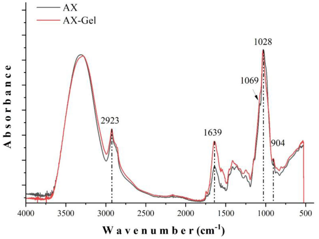
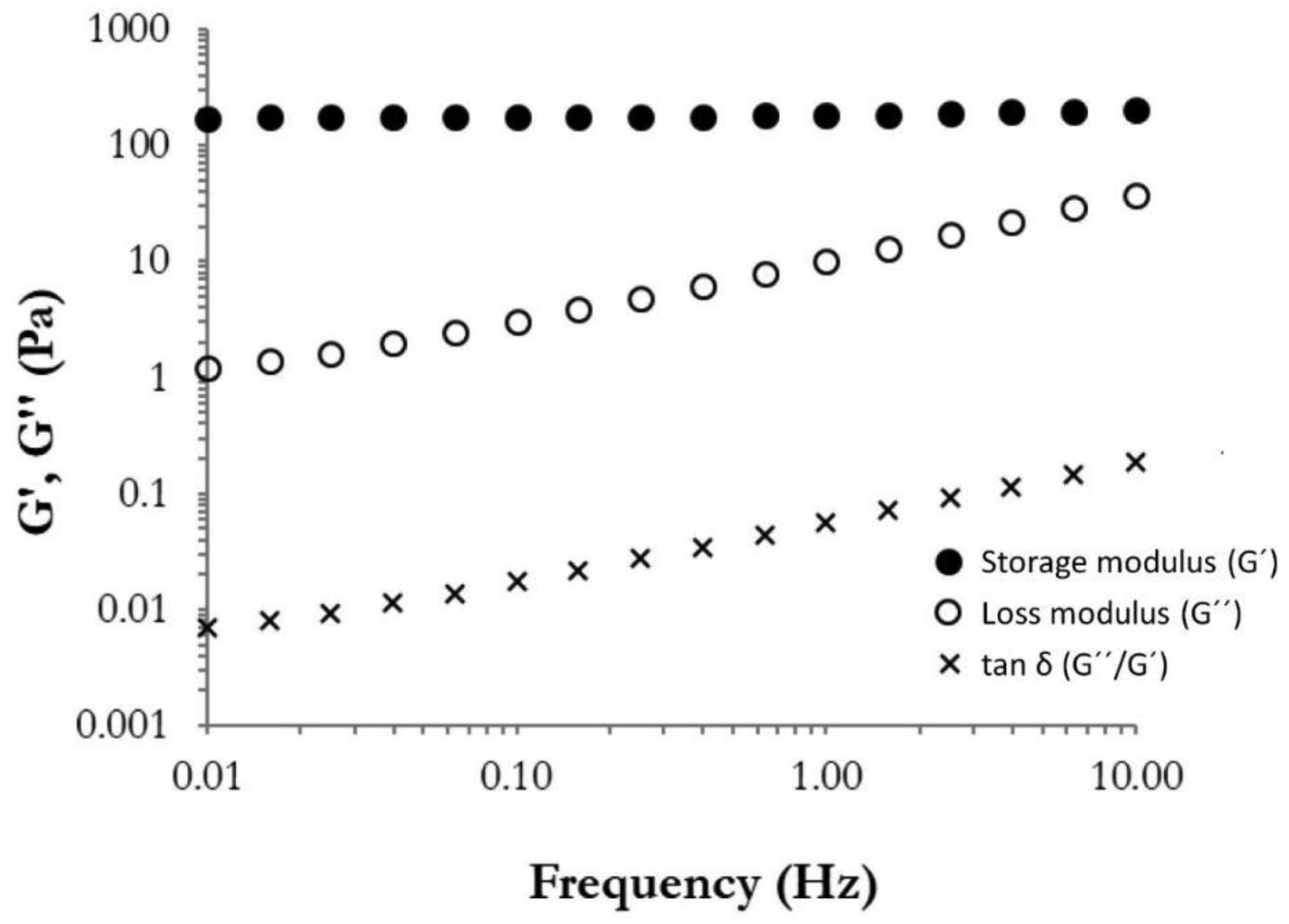
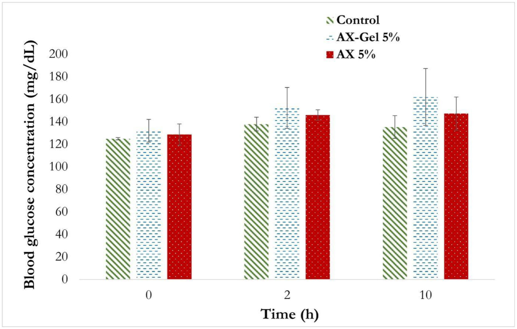
Several studies have described the health benefits of arabinoxylan as prebiotics; however, other authors have related them with an anti-nutrient effect as arabinoxylan increases the viscosity of the alimentary bolus. In this work, the impact of arabinoxylan and crosslinked arabinoxylan on blood serum lipids and glucose levels of Wistar rats was investigated. Arabinoxylan was extracted from maize bran, presented a Fourier Transform Infra-Red spectrum typical for this polysaccharide, and a molecular weight of 250 kDa. Arabinoxylan solution at 4% (w/v) formed covalent gels induced by laccase. Male Wistar rats were fed a standard diet supplemented with 5% (w/w) lyophilized arabinoxylan or crosslinked arabinoxylan. Blood glucose levels were determined, collecting a drop of blood from the tail vein of rats at 0, 2, and 10 h after food consumption. Total cholesterol, triglycerides, high-density lipoprotein (HDL) cholesterol, and low-density lipoprotein (LDL) cholesterol were also determined. Postprandial blood glucose of the treatment groups was maintained at the same level as the control group. The serum lipid profile levels also remained close to the control group, excepting total cholesterol and LDL-cholesterol, which were higher in crosslinked arabinoxylan treatment but in the range reported for this murine model. The obtained results revealed that consumption of arabinoxylan and crosslinked arabinoxylan at moderated levels does not interfere with the absorption of these nutrients.
Citation: Figueroa-Pizano María Dolores, Campa-Mada Alma Consuelo, Canett-Romero Rafael, Paz-Samaniego Rita, Martínez-López Ana Luisa, Carvajal-Millan Elizabeth. Influence of arabinoxylan and crosslinked arabinoxylan consumption on blood serum lipids and glucose levels of Wistar rats[J]. AIMS Bioengineering, 2021, 8(3): 208-220. doi: 10.3934/bioeng.2021018
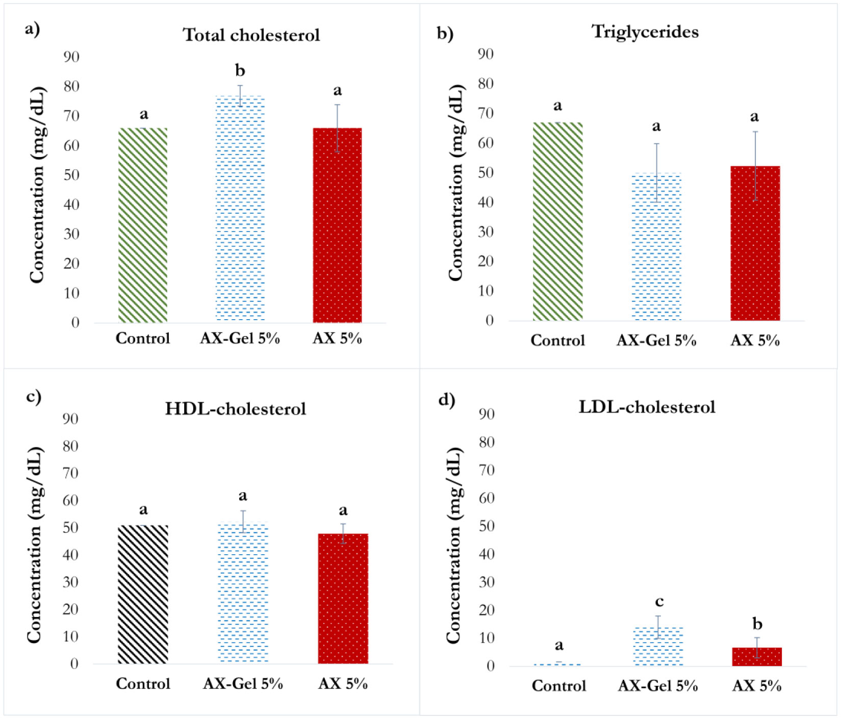
Several studies have described the health benefits of arabinoxylan as prebiotics; however, other authors have related them with an anti-nutrient effect as arabinoxylan increases the viscosity of the alimentary bolus. In this work, the impact of arabinoxylan and crosslinked arabinoxylan on blood serum lipids and glucose levels of Wistar rats was investigated. Arabinoxylan was extracted from maize bran, presented a Fourier Transform Infra-Red spectrum typical for this polysaccharide, and a molecular weight of 250 kDa. Arabinoxylan solution at 4% (w/v) formed covalent gels induced by laccase. Male Wistar rats were fed a standard diet supplemented with 5% (w/w) lyophilized arabinoxylan or crosslinked arabinoxylan. Blood glucose levels were determined, collecting a drop of blood from the tail vein of rats at 0, 2, and 10 h after food consumption. Total cholesterol, triglycerides, high-density lipoprotein (HDL) cholesterol, and low-density lipoprotein (LDL) cholesterol were also determined. Postprandial blood glucose of the treatment groups was maintained at the same level as the control group. The serum lipid profile levels also remained close to the control group, excepting total cholesterol and LDL-cholesterol, which were higher in crosslinked arabinoxylan treatment but in the range reported for this murine model. The obtained results revealed that consumption of arabinoxylan and crosslinked arabinoxylan at moderated levels does not interfere with the absorption of these nutrients.
arabinoxylan
crosslinked arabinoxylan
ferulic acid
high-density lipoprotein
low-density lipoprotein
arabinose to xylose ratio
Fourier transform infrared
potassium bromide
Research Center for Food and Development
storage modulus
loss modulus

| [1] |
Fadel A, Mahmoud AM, Ashworth JJ, et al. (2018) Health-related effects and improving extractability of cereal arabinoxylans. Int J Biol Macromol 109: 819-831. doi: 10.1016/j.ijbiomac.2017.11.055

|
| [2] |
Van Den Abbeele P, Venema K, Van De Wiele T, et al. (2013) Different human gut models reveal the distinct fermentation patterns of arabinoxylan versus inulin. J Agric Food Chem 61: 9819-9827. doi: 10.1021/jf4021784
|
| [3] |
Chen Z, Li S, Fu Y, et al. (2019) Arabinoxylan structural characteristics, interaction with gut microbiota and potential health functions. J Funct Foods 54: 536-551. doi: 10.1016/j.jff.2019.02.007
|
| [4] | Mendez-Encinas MA, Carvajal-Millan E, Rascon-Chu A, et al. (2018) Ferulated arabinoxylans and their gels: Functional properties and potential application as antioxidant and anticancer agent. Oxid Med Cell Longev 2018: 2314759. |
| [5] | Méndez-Encinas MA, Carvajal-Millan E, Rascón-Chu A, et al. (2019) Arabinoxylans and the remaining protein fraction relationship with the gelling capability of the polysaccharide. Acta Univ 29: 1-19. |
| [6] | Morales-ortega A, Niño-medina G, Carvajal-millán E, et al. (2013) Ferulated arabinoxylans from cereals: A review of their physico-chemical characteristics and gelling capability. Rev Fitotec Mex 36: 439-446. |
| [7] |
Niño-Medina G, Carvajal-Millan E, Rascon-Chu A, et al. (2010) Feruloylated arabinoxylans and arabinoxylan gels: structure, sources and applications. Phytochem Rev 9: 111-120. doi: 10.1007/s11101-009-9147-3
|
| [8] |
Nie Q, Chen H, Hu J, et al. (2018) Arabinoxylan attenuates type 2 diabetes by improvement of carbohydrate, lipid, and amino acid metabolism. Mol Nutr Food Res 62: 1800222. doi: 10.1002/mnfr.201800222
|
| [9] |
Carvajal-Millan E, Vargas-Albores F, Fierro-Islas JM, et al. (2020) Arabinoxylans and gelled arabinoxylans used as anti-obesogenic agents could protect the stability of intestinal microbiota of rats consuming high-fat diets. Int J Food Sci Nutr 71: 74-83. doi: 10.1080/09637486.2019.1610729
|
| [10] |
Mendis M, Simsek S (2014) Arabinoxylans and human health. Food Hydrocoll 42: 239-243. doi: 10.1016/j.foodhyd.2013.07.022
|
| [11] |
Izydorczyk MS, Biliaderis CG (1995) Cereal arabinoxylans: advances in structure and physicochemical properties. Carbohydr Polym 28: 33-48. doi: 10.1016/0144-8617(95)00077-1
|
| [12] | Anderson C, Simsek S (2018) What are the characteristics of arabinoxylan gels? Food Nutr Sci 09: 818-833. |
| [13] |
Hopkins MJ, Englyst HN, Macfarlane S, et al. (2003) Degradation of cross-linked and non-cross-linked arabinoxylans by the intestinal microbiota in children. Appl Environ Microbiol 69: 6354-6360. doi: 10.1128/AEM.69.11.6354-6360.2003
|
| [14] |
Möhlig M, Koebnick C, Weickert MO, et al. (2005) Arabinoxylan-enriched meal increases serum ghrelin levels in healthy humans. Horm Metab Res 37: 303-308. doi: 10.1055/s-2005-861474
|
| [15] |
Hartvigsen ML, Gregersen S, Lærke HN, et al. (2014) Effects of concentrated arabinoxylan and β-glucan compared with refined wheat and whole grain rye on glucose and appetite in subjects with the metabolic syndrome: a randomized study. Eur J Clin Nutr 68: 84-90. doi: 10.1038/ejcn.2013.236
|
| [16] |
Shelat KJ, Vilaplana F, Nicholson TM, et al. (2010) Diffusion and viscosity in arabinoxylan solutions: implications for nutrition. Carbohydr Polym 82: 46-53. doi: 10.1016/j.carbpol.2010.04.019
|
| [17] |
Malunga LN, Izydorczyk M, Beta T (2017) Antiglycemic effect of water extractable arabinoxylan from wheat aleurone and bran. J Nutr Metab 2017: 5784759. doi: 10.1155/2017/5784759
|
| [18] |
Hartvigsen ML, Jeppesen PB, Lærke HN, et al. (2013) Concentrated arabinoxylan in wheat bread has beneficial effects as rye breads on glucose and changes in gene expressions in insulin-sensitive tissues of Zucker diabetic fatty (ZDF) rats. J Agric Food Chem 61: 5054-5063. doi: 10.1021/jf3043538
|
| [19] |
Zarghi H (2018) Application of xylanas and β-glucanase to improve nutrient utilization in poultry fed cereal base diets: Used of enzymes in poultry diet. Insights Enzym Res 2: 11-17. doi: 10.21767/2573-4466.100011
|
| [20] |
Yaghobfar A, Kalantar M (2017) Effect of non-starch polysaccharide (NSP) of wheat and barley supplemented with exogenous enzyme blend on growth performance, gut microbial, pancreatic enzyme activities, expression of glucose transporter (SGLT1) and mucin producer (MUC2) genes of broiler chickens. Rev Bras Ciência Avícola 19: 629-638. doi: 10.1590/1806-9061-2016-0441
|
| [21] |
Carvajal-Millan E, Rascón-Chu A, Márquez-Escalante JA, et al. (2007) Maize bran gum: Extraction, characterization and functional properties. Carbohydr Polym 69: 280-285. doi: 10.1016/j.carbpol.2006.10.006
|
| [22] |
Martínez-López AL, Carvajal-Millan E, Rascón-Chu A, et al. (2013) Gels of ferulated arabinoxylans extracted from nixtamalized and non-nixtamalized maize bran: rheological and structural characteristics. CYTA - J Food 11: 22-28. doi: 10.1080/19476337.2013.781679
|
| [23] |
Morales-Ortega A, Carvajal-Millan E, López-Franco Y, et al. (2013) Characterization of water extractable arabinoxylans from a spring wheat flour: rheological properties and microstructure. Molecules 18: 8417-8428. doi: 10.3390/molecules18078417
|
| [24] |
Berlanga-Reyes CM, Carvajal-Millán E, Lizardi-Mendoza J, et al. (2009) Maize arabinoxylan gels as protein delivery matrices. Molecules 14: 1475-1482. doi: 10.3390/molecules14041475
|
| [25] |
Martínez-López AL, Carvajal-Millan E, Miki-Yoshida M, et al. (2013) Arabinoxylan microspheres: structural and textural characteristics. Molecules 18: 4640-4650. doi: 10.3390/molecules18044640
|
| [26] |
Paz-Samaniego R, Carvajal-Millan E, Sotelo-Cruz N, et al. (2016) Maize processing waste water upcycling in Mexico: Recovery of arabinoxylans for probiotic encapsulation. Sustain 8: 1104. doi: 10.3390/su8111104
|
| [27] |
González-Estrada R, Calderón-Santoyo M, Carvajal-Millan E, et al. (2015) Covalently cross-linked arabinoxylans films for Debaryomyces hansenii entrapment. Molecules 20: 11373-11386. doi: 10.3390/molecules200611373
|
| [28] |
Li L, Ma S, Fan L, et al. (2016) The influence of ultrasonic modification on arabinoxylans properties obtained from wheat bran. Int J Food Sci Technol 51: 2338-2344. doi: 10.1111/ijfs.13239
|
| [29] |
Martínez-López AL, Carvajal-millan E, Sotelo-cruz N, et al. (2019) Enzymatically cross-linked arabinoxylan microspheres as oral insulin delivery system. Int J Biol Macromol 126: 952-959. doi: 10.1016/j.ijbiomac.2018.12.192
|
| [30] |
Paz-Samaniego R, Rascón-Chu A, Brown-Bojorquez F, et al. (2018) Electrospray-assisted fabrication of core-shell arabinoxylan gel particles for insulin and probiotics entrapment. J Appl Polym Sci 135: 46411. doi: 10.1002/app.46411
|
| [31] |
Morales-Burgos AM, Carvajal-millan E, López-Franco YL, et al. (2017) Syneresis in gels of highly ferulated arabinoxylans: characterization of covalent cross-linking, rheology, and microstructure. Polymers 9: 164. doi: 10.3390/polym9050164
|
| [32] |
Berlanga-Reyes CM, Carvajal-Millan E, Lizardi-Mendoza J, et al. (2011) Enzymatic cross-linking of alkali extracted arabinoxylans: Gel rheological and structural characteristics. Int J Mol Sci 12: 5853-5861. doi: 10.3390/ijms12095853
|
| [33] |
Kale MS, Hamaker BR, Campanella OH (2013) Alkaline extraction conditions determine gelling properties of corn bran arabinoxylans. Food Hydrocoll 31: 121-126. doi: 10.1016/j.foodhyd.2012.09.011
|
| [34] |
Marquez-Escalante JA, Carvajal-Millan E, Yadav MP, et al. (2018) Rheology and microstructure of gels based on wheat arabinoxylans enzymatically modified in arabinose to xylose ratio. J Sci Food Agric 98: 914-922. doi: 10.1002/jsfa.8537
|
| [35] |
Marquez-Escalante JA, Carvajal-Millan E (2019) Feruloylated arabinoxylans from Maize Distiller's dried grains with solubles: Effect of feruloyl esterase on their macromolecular characteristics, gelling, and antioxidant properties. Sustain 11: 6449. doi: 10.3390/su11226449
|
| [36] |
Mendez-Encinas MA, Carvajal-Millan E, Yadav MP, et al. (2019) Partial removal of protein associated with arabinoxylans: Impact on the viscoelasticity, crosslinking content, and microstructure of the gels formed. J Appl Polym Sci 136: 47300. doi: 10.1002/app.47300
|
| [37] |
Vansteenkiste E, Babot C, Rouau X, et al. (2004) Oxidative gelation of feruloylated arabinoxylan as affected by protein. Influence on protein enzymatic hydrolysis. Food Hydrocoll 18: 557-564. doi: 10.1016/j.foodhyd.2003.09.004
|
| [38] | Ross-Murphy SB (1984) Rheological methods. Biophysical Methods in Food Research Oxford: Blackwell Scientific Publishing, 138-199. |
| [39] |
Vogel B, Gallaher DD, Bunzel M (2012) Influence of cross-linked arabinoxylans on the postprandial blood glucose response in rats. J Agric Food Chem 60: 3847-3852. doi: 10.1021/jf203930a
|
| [40] |
Li S, Liu M, Chen Z, et al. (2021) Cross-linking treatment of arabinoxylan improves its antioxidant and hypoglycemic activities after simulated in vitro digestion. Lwt 145: 111386. doi: 10.1016/j.lwt.2021.111386
|
| [41] |
Nielsen TS, Theil PK, Purup S, et al. (2015) Effects of resistant starch and arabinoxylan on parameters related to large intestinal and metabolic health in pigs fed fat-rich diets. J Agric Food Chem 63: 10418-10430. doi: 10.1021/acs.jafc.5b03372
|
| [42] |
Pluschke AM, Williams BA, Zhang D, et al. (2018) Male grower pigs fed cereal soluble dietary fibres display biphasic glucose response and delayed glycaemic response after an oral glucose tolerance test. PLoS One 13: e0193137. doi: 10.1371/journal.pone.0193137
|
| [43] |
Giulia Falchi A, Grecchi I, Muggia C, et al. (2016) Effects of a Bioavailable Arabinoxylan-enriched White Bread Flour on Postprandial Glucose Response in Normoglycemic Subjects. J Diet Suppl 13: 626-633. doi: 10.3109/19390211.2016.1156798
|
| [44] |
Garcia AL, Otto B, Reich SC, et al. (2007) Arabinoxylan consumption decreases postprandial serum glucose, serum insulin and plasma total ghrelin response in subjects with impaired glucose tolerance. Eur J Clin Nutr 61: 334-341. doi: 10.1038/sj.ejcn.1602525
|
| [45] | Harini M, Astirin OP (2009) Blood cholesterol levels of hypercholesterolemic rat (Rattus norvegicus) after VCO treatment. Nusant Biosci 1: 53-58. |
| [46] | Sa'adah NN, Purwani KI, Nurhayati APD, et al. (2016) Analysis of lipid profile and atherogenic index in hyperlipidemic rat (Rattus norvegicus Berkenhout, 1769) that given the methanolic extract of Parijoto (Medinilla speciosa). Proceeding of International Biology Conference 020031. |
| [47] |
Oyeyemi AW, Ugwuezumba PC, Daramola OO, et al. (2019) Comparative effects of Zea mays bran, Telfairia occidentalis and Citrus sinensis feeds on bowel transit rate, postprandial blood glucose and lipids profile in male wistar rats. Niger J Basic Appl Sci 26: 80-87. doi: 10.4314/njbas.v26i1.9
|
| [48] |
Chen H, Fu Y, Jiang X, et al. (2018) Arabinoxylan activates lipid catabolism and alleviates liver damage in rats induced by high-fat diet. J Sci Food Agric 98: 253-260. doi: 10.1002/jsfa.8463
|
| [49] |
Gunness P, Williams BA, Gerrits WJJ, et al. (2016) Circulating triglycerides and bile acids are reduced by a soluble wheat arabinoxylan via modulation of bile concentration and lipid digestion rates in a pig model. Mol Nutr Food Res 60: 642-651. doi: 10.1002/mnfr.201500686
|
| [50] |
Schioldan AG, Gregersen S, Hald S, et al. (2018) Effects of a diet rich in arabinoxylan and resistant starch compared with a diet rich in refined carbohydrates on postprandial metabolism and features of the metabolic syndrome. Eur J Nutr 57: 795-807. doi: 10.1007/s00394-016-1369-8
|
| [51] |
Lu ZX, Walker KZ, Muir JG, et al. (2004) Arabinoxylan fibre improves metabolic control in people with type II diabetes. Eur J Clin Nutr 58: 621-628. doi: 10.1038/sj.ejcn.1601857
|
| [52] | Colpo A (2005) LDL cholesterol: bad cholesterol, or bad science? J Am Physicians Surg 10: 83. |
Figures(5) / Tables(1)

Figueroa-Pizano María Dolores, Campa-Mada Alma Consuelo, Canett-Romero Rafael, Paz-Samaniego Rita, Martínez-López Ana Luisa, Carvajal-Millan Elizabeth. Influence of arabinoxylan and crosslinked arabinoxylan consumption on blood serum lipids and glucose levels of Wistar rats[J]. AIMS Bioengineering, 2021, 8(3): 208-220. doi: 10.3934/bioeng.2021018


 DownLoad: