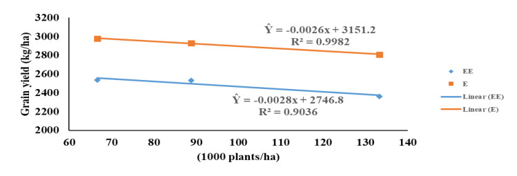
Maize (Zea mays L.) breeders in the West and Central Africa have developed and commercialized extra-early and early-maturing maize hybrids, which combine high yield potentials with tolerance/resistance to drought, low soil-N and Striga infestation. Hybrids of both maturity groups have not been investigated for tolerance to high plant density and N application and are new to the farmers; thus, the urgent need to recommend appropriate agronomic practices for these hybrids. We investigated the responses of four hybrids, belonging to the extra-early and early-maturity groups, to three plant densities and three N rates in five locations of different agroecologies. The early-maturing hybrids consistently out-yielded the extra-early maturing hybrids in all the five agroecologies. The hybrids showed no response to N-fertilizer application above 90 kg ha−1. All interactions involving N had no significant effect on grain yield and other measured agronomic traits except in few cases. The extra-early and early-maturing hybrids had similar response to plant density; their grain yield decreased as density increased. Contrarily, flowering was delayed and expression of some other agronomic traits such as plant and ear aspects were negatively impacted by increased density. Optimal yield for hybrids of both maturity groups was obtained at approximately 90 kg N ha−1 and 66,666 plants ha−1. Most of the measured traits indicated high repeatability estimates across the N levels, densities and environments. Evidently, the hybrids were intolerant of elevated density. It therefore, becomes necessary to improve maize germplasms for high plant density tolerance in the region.
Citation: Babatope Samuel Ajayo, Baffour Badu-Apraku, Morakinyo A. B. Fakorede, Richard O. Akinwale. Plant density and nitrogen responses of maize hybrids in diverse agroecologies of west and central Africa[J]. AIMS Agriculture and Food, 2021, 6(1): 381-400. doi: 10.3934/agrfood.2021023
Maize (Zea mays L.) breeders in the West and Central Africa have developed and commercialized extra-early and early-maturing maize hybrids, which combine high yield potentials with tolerance/resistance to drought, low soil-N and Striga infestation. Hybrids of both maturity groups have not been investigated for tolerance to high plant density and N application and are new to the farmers; thus, the urgent need to recommend appropriate agronomic practices for these hybrids. We investigated the responses of four hybrids, belonging to the extra-early and early-maturity groups, to three plant densities and three N rates in five locations of different agroecologies. The early-maturing hybrids consistently out-yielded the extra-early maturing hybrids in all the five agroecologies. The hybrids showed no response to N-fertilizer application above 90 kg ha−1. All interactions involving N had no significant effect on grain yield and other measured agronomic traits except in few cases. The extra-early and early-maturing hybrids had similar response to plant density; their grain yield decreased as density increased. Contrarily, flowering was delayed and expression of some other agronomic traits such as plant and ear aspects were negatively impacted by increased density. Optimal yield for hybrids of both maturity groups was obtained at approximately 90 kg N ha−1 and 66,666 plants ha−1. Most of the measured traits indicated high repeatability estimates across the N levels, densities and environments. Evidently, the hybrids were intolerant of elevated density. It therefore, becomes necessary to improve maize germplasms for high plant density tolerance in the region.

| [1] | Badu-Apraku B, Menkir A, Fakorede MAB, et al. (2006) Multivariate analysis of the genetic diversity of forty-seven Striga resistant tropical early maturing maize inbred lines. Maydica 51: 551–559. |
| [2] | FAOSTAT (2020) Production: Crop Statistics, Cereal Category. Food and Agricultural commodities production. Food and Agriculture Organization of the United Nations Statistics (FAOSTAT). |
| [3] | Badu-Apraku B, Oyekunle M, Akinwale RO (2013) Breakthroughs in maize breeding. IITA, Ibadan, Nigeria; and R.O. Akinwale, Obafemi Awolowo, University, Ile-Ife, Nigeria. |
| [4] | Byerlee D, Eicher C (1971) Africa's emerging maize revolution. Boulder, Colorado, Lynee Rienner. |
| [5] | Badu-Apraku B, Akinwale RO, Fakorede MAB (2010) Selection of early maturing maize inbred lines for hybrid production using multiple traits under Striga-infested and Striga-free environments. Maydica 55: 261–274. |
| [6] | Badu-Apraku B, Fakorede MAB (2017) Breeding for Tolerance to Low Soil Nitrogen. In: Badu-Apraku B, Fakorede MAB (Eds.), Advances in Genetic Enhancement of Early and Extra-Early Maize for Sub-Saharan Africa, Cham, Springer International Publishing, 359–378. |
| [7] |
Akinwale RO, Badu-Apraku B, Fakorede MAB, et al. (2014) Heterotic grouping of tropical early-maturing maize inbred lines based on combining ability in Striga-infested and Striga-free environments and the use of SSR markers for genotyping. Field Crops Res 156: 48–62. doi: 10.1016/j.fcr.2013.10.015

|
| [8] |
Badu-Apraku B, Talabi AO, Ifie BE, et al. (2018) Gains in grain yield of extra-early maize during three breeding periods under drought and rainfed conditions. Crop Sci 58: 2399–2412. doi: 10.2135/cropsci2018.03.0168
|
| [9] | Kamara AY (2013) Best practices for maize production in the West African savannas. Ibadan, Nigeria, International Institute of Tropical Agriculture (IITA). |
| [10] | Sangoi L (2001) Understanding plant density effects on maize growth and development: An important issue to maximize grain yield. Ciencia Rural 31 no.1. |
| [11] |
Iken JE, Amusa NA (2004) Maize research and production in Nigeria. Afr J Biotechnol 3: 302–307. doi: 10.5897/AJB2004.000-2056
|
| [12] | Kamara AY, Ekeleme F, Omoigui L, et al. (2009) Influence of nitrogen fertilization on the performance of early and late maturing maize varieties under natural infestation with Striga hermonthica (Del.) Benth. Arch Agron Soil Sci 55: 125–145. |
| [13] | Druilhe Z, Barreiro-hurlé J (2012) Fertilizer subsidies in sub-Saharan Africa. ESA Working Papers No. 12-04, Agricultural Development Economics Division Food and Agriculture Organization of the United Nations. |
| [14] | Mansfield BD, Mumm RH (2014) Survey of plant density tolerance in U.S. maize germplasm. Crop Sci 54: 157–173. |
| [15] |
Yan P, Pan J, Zhang W, et al. (2017) A high plant density reduces the ability of maize to use soil nitrogen. PLoS One 12: e0172717. doi: 10.1371/journal.pone.0172717
|
| [16] | Babaji BA, Ibrahim YB, Mahadi MA, et al. (2012) Response of extra-early maize (Zea mays L.) to varying intra-row spacing and hill density. Global J Bio-Sci Biotechnol 1: 110–115. |
| [17] | Sharifai AI, Mahmud M, Tanimu B, et al. (2012) Yield and Yield componemts of extra early maize (zea mays L.) as influenced by intra-row spacing, nitrogen and poultry manure rates. Bayero J Pure Appl Sci 5: 113–122. |
| [18] | Westgate ME (1994) Seed formation in maize during drought. In: Boote KJ, Bennett JM, Sinclair TR, Physiology and determination of crop yield, 361–364. |
| [19] |
Herrero MP, Johnson RR (1981) Drought stress and its effects on maize reproductive systems. Crop Sci 21: 105–110. doi: 10.2135/cropsci1981.0011183X002100010029x
|
| [20] |
Edmeades GO, Bolaños J, Hernandez M, et al. (1993) Causes for silk delay in a lowland tropical maize population. Crop Sci 33: 1029–1035. doi: 10.2135/cropsci1993.0011183X003300050031x
|
| [21] |
Badu-Apraku B, Fakorede MAB, Annor B, et al. (2018) Improvement in grain yield and low-nitrogen tolerance in maize cultivars of three eras. Exp Agric 54: 805–823. doi: 10.1017/S0014479717000394
|
| [22] | MIP (2017) Maize Improvement Program, Drought tolerant maize varieties released under DTMA in Nigeria, Mali and Ghana from 2007–2016. Ibadan, Nigeria., International Institute of Tropical Agriculture (IITA). |
| [23] | SAS Institute (2002) SAS User's Guide. Version 9.0, Cary, NC: SAS Institute Inc., Statistical Analysis System (SAS) Institute. |
| [24] | Fehr W (1991) Principles of Cultivar Development: Theory and Technique. Agronomy Books 1. |
| [25] | Falconer DS, Mackay TFC (1996) Introduction to Quantitative Genetics 4th edition Longman Scientific & Technical, New York, NY. |
| [26] |
Bello OB, Abdulmaliq SY, Ige S, et al. (2012) Evaluation of early and late/intermediate maize varieties for grain yield potential and adaptation to a southern guinea savanna agro-ecology of Nigeria. Int J Plant Res 2: 14–21. doi: 10.5923/j.plant.20120202.03
|
| [27] | Oluwaranti A, Fakorede MAB, Badu-Apraku B (2008) Grain yield of maize varieties of different maturity groups under marginal rainfall conditions. J Agric Sci (Belgrade) 53: 183–191. |
| [28] | Oluwaranti A, Fakorede MAB, Adeboye FA (2015) Maturity groups and phenology of maize in a rainforest location. Int J Agric Innovations Res 4: 124–127. |
| [29] |
Edwards JW (2016) Genotype × Environment interaction for plant density response in maize (Zea mays L.). Crop Sci 56: 1493–1505. doi: 10.2135/cropsci2015.07.0408
|
| [30] |
Oyekunle M, Haruna A, Badu-Apraku B, et al. (2017) Assessment of early-maturing maize hybrids and testing sites using GGE Biplot analysis. Crop Sci 57: 2942–2950. doi: 10.2135/cropsci2016.12.1014
|
| [31] | Badu-Apraku B, Fakorede B, Akinwale R, et al. (2020) Application of the GGE Biplot as a statistical tool in the breeding and testing of early and extra-early maturing maize in sub-Saharan Africa. Crop Breed Genet Genom 2: e200012. |
| [32] | Abayomi YA, Awokola CD, Lawal Z (2012) Comparative evaluation of water deficit tolerance capacity of extra-early and early maize genotypes under controlled conditions. J Agric Sci 4: 54–71. |
| [33] | Badu-Apraku B, Fakorede MAB (2017) Improvement of early and extra-early maize for combined tolerance to drought and heat stress in sub-Saharan Africa. In: Badu-Apraku B, Fakorede MAB (Eds.), Advances in Genetic Enhancement of Early and Extra-Early Maize for Sub-Saharan Africa, Cham, Springer International Publishing, 311–358. |
| [34] | Badu-Apraku B, Fakorede MAB (2017) Climatology of Maize in Sub-Saharan Africa. In: Badu-Apraku B, Fakorede MAB (Eds.), Advances in Genetic Enhancement of Early and Extra-Early Maize for Sub-Saharan Africa, Cham, Springer International Publishing, 11–31. |
| [35] |
Esechie HA, Rodriguez V, Al-Asmi H (2004) Comparison of local and exotic maize varieties for stalk lodging components in a desert climate. Eur J Agron 21: 21–30. doi: 10.1016/S1161-0301(03)00060-1
|
| [36] | Salami AE, Adegoke SAO, Adegbite OA (2007) Genetic variability among maize cultivars grown in Ekiti-State, Nigeria. Middle-East J Sci Res 2: 09–13. |
| [37] | Ahmad S, Khan AA, Kamran M, et al. (2018) Response of Maize Cultivars to Various Nitrogen Levels. Eur J Exp Bio 8: No1:2. |
| [38] |
Al-Naggar A, Shabana R, Atta M, et al. (2015) Matching the optimum plant density and adequate N-rate with high-density tolerant genotype for maxmizing maize (Zea mays L.) crop yield. JAERI 2: 237–253. doi: 10.9734/JAERI/2015/14260
|
| [39] |
Qian C, Yu Y, Gong X, et al. (2016) Response of grain yield to plant density and nitrogen rate in spring maize hybrids released from 1970 to 2010 in Northeast China. Crop J 4: 459–467. doi: 10.1016/j.cj.2016.04.004
|
| [40] | Worku A, Derebe B, Bitew Y, et al. (2020) Response of maize (Zea mays L.) to nitrogen and planting density in Jabitahinan district, Western Amhara region. Cogent Food & Agric 6: 1770405. |
| [41] |
Mastrodomenico AT, Haegele JW, Seebauer JR, et al. (2018) Yield stability differs in commercial maize hybrids in response to changes in plant density, nitrogen fertility, and environment. Crop Sci 58: 230–241. doi: 10.2135/cropsci2017.06.0340
|
| [42] |
Badu-Apraku B, Fakorede MAB, Gedil M, et al. (2016) Heterotic patterns of IITA and CIMMYT early-maturing yellow maize inbreds under contrasting environments. Agron J 108: 1321–1336. doi: 10.2134/agronj2015.0425
|
| [43] | Al-Naggar AMM, Atta MMM, Ahmed MA, et al. (2016) Genetic parameters controlling inheritance of agronomic and yield traits of maize (Zea mays L.) under elevated plant density. J Adv Biol & Biotechnol 9: 1–19. |
| [44] | Shrestha J (2013) Effect of nitrogen and plant population on flowering and grain yield of winter maize. Sky J Agric Res 2: 64–68. |
| [45] | Al-Naggar AMM, Atta MMM (2017) Elevated plant density effects on performance and genetic parameters controlling maize (Zea mays L.) agronomic traits. J Adv Biol & Biotechnol 12: 1–20. |
| [46] |
Kamara MM, Rehan M, Ibrahim KM, et al. (2020) Genetic diversity and combining ability of white maize inbred lines under different plant densities. Plants 9: 1140. doi: 10.3390/plants9091140
|
| [47] | Fakorede MAB, Kim S, Mareck J, et al. (1989) Breeding Strategies and Potentials of available varieties in relation to attaining self-sufficiency in maize production in Nigeria. Presented at the National Symposium "Towards the attainment of Self-Sufficiency of Maize Production" in Nigeria, Ibadan. |
| [48] |
Badu-Apraku B, Akinwale RO, Ajala SO, et al. (2011) Relationships among traits of tropical early maize cultivars in contrasting environments. Agron J 103: 717–729. doi: 10.2134/agronj2010.0484
|
| [49] |
Oyekunle M, Badu-Apraku B (2014) Genetic analysis of grain yield and other traits of early-maturing maize inbreds under drought and well-watered conditions. J Agron Crop Sci 200: 92–107. doi: 10.1111/jac.12049
|
Figures(1) / Tables(7)

Babatope Samuel Ajayo, Baffour Badu-Apraku, Morakinyo A. B. Fakorede, Richard O. Akinwale. Plant density and nitrogen responses of maize hybrids in diverse agroecologies of west and central Africa[J]. AIMS Agriculture and Food, 2021, 6(1): 381-400. doi: 10.3934/agrfood.2021023


 DownLoad: