Analysis of a fractional pollution model in a system of three interconnecting lakes

Yasir Nadeem Anjam; Mehmet Yavuz; Mati ur Rahman; Amna Batool; Yasir Nadeem Anjam; Mehmet Yavuz; Mati ur Rahman; Amna Batool

doi:10.3934/biophy.2023014

AIMS Biophysics

2023, Volume 10, Issue 2: 220-240. doi: 10.3934/biophy.2023014

Previous Article Next Article

Research article Special Issues

Analysis of a fractional pollution model in a system of three interconnecting lakes

1.
Department of Applied Sciences, National Textile University, Faisalabad 37610, Pakistan
2.
Department of Mathematics, Environment & Sustainability Institute, College of Engineering, Mathematics & Physical Sciences, University of Exeter-Penryn Campus, TR10, UK
3.
Necmettin Erbakan University, Department of Mathematics and Computer Sciences, Meram Yeniyol, 42090 Meram, Konya, Türkiye
4.
School of Mathematical Science, Shanghai Jiao Tong University, P.R. China
5.
Department of Computer Science and Mathematics, Lebanese American University, Beirut, Lebanon

Received: 10 February 2023 Revised: 18 May 2023 Accepted: 24 May 2023 Published: 31 May 2023

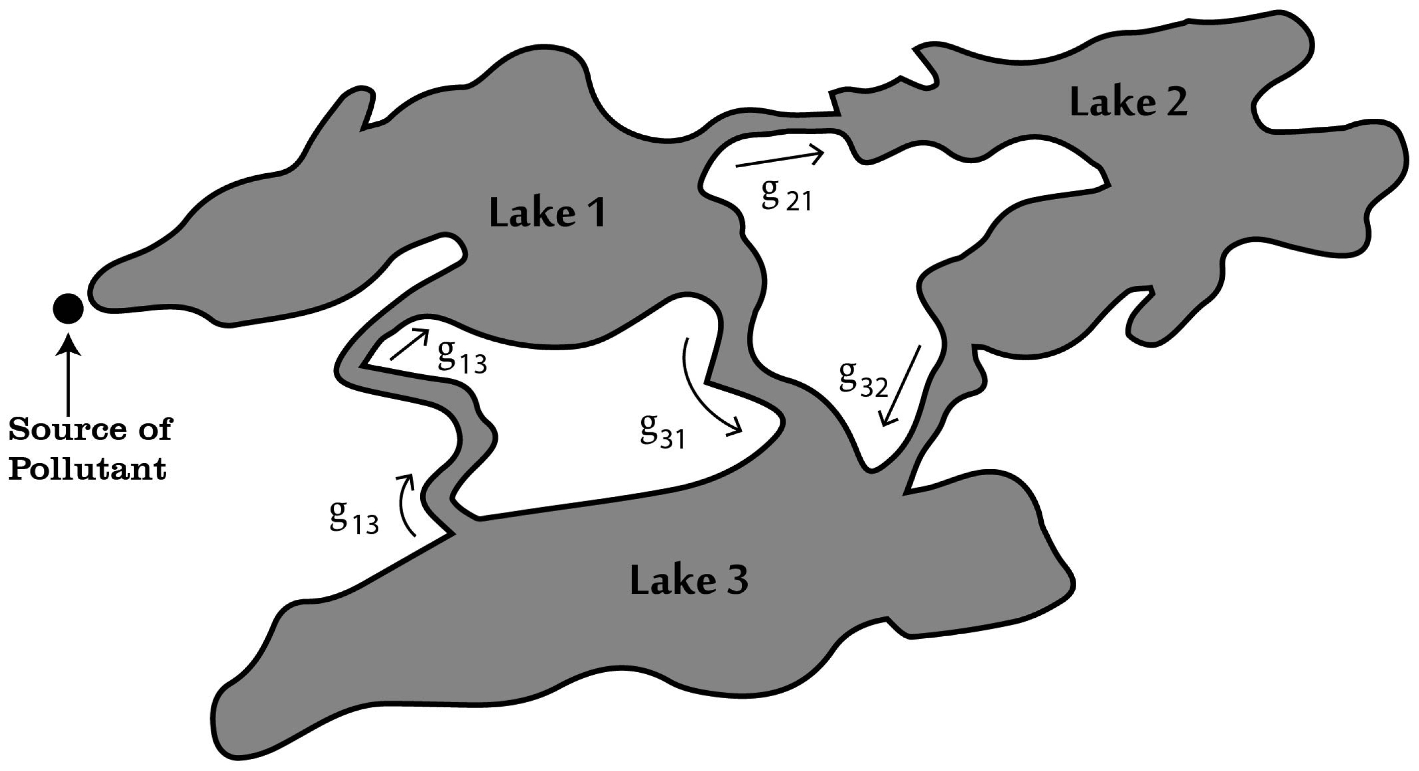
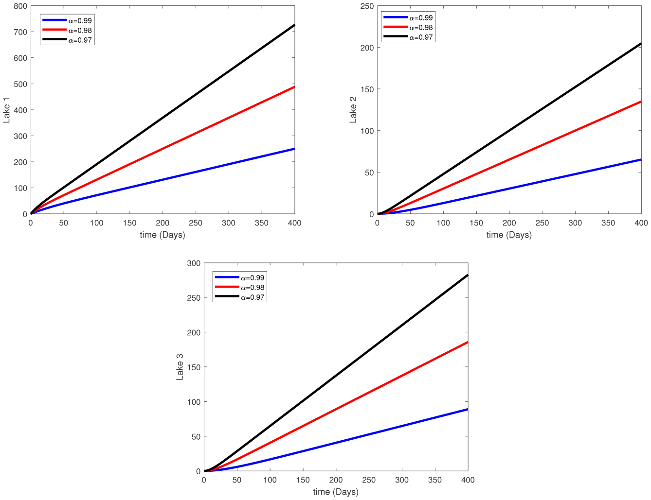
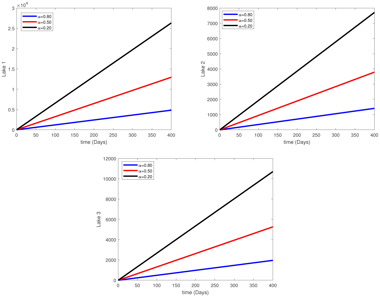
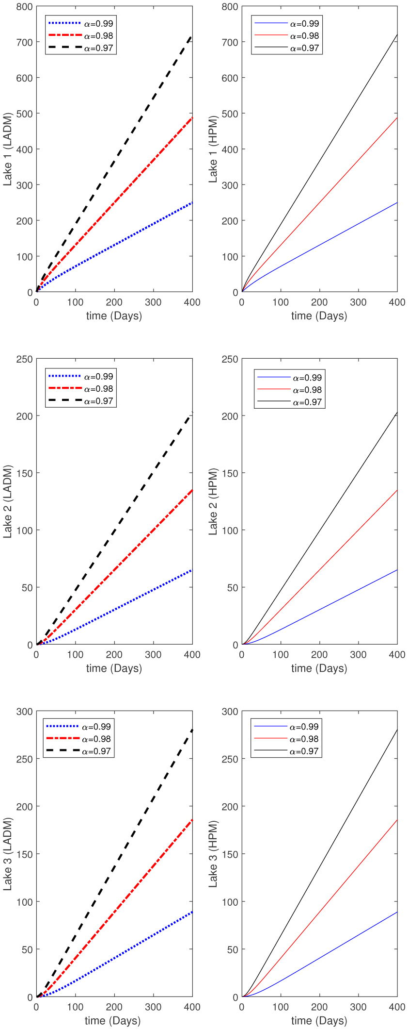
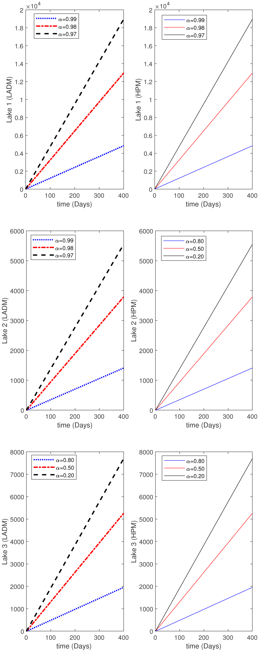
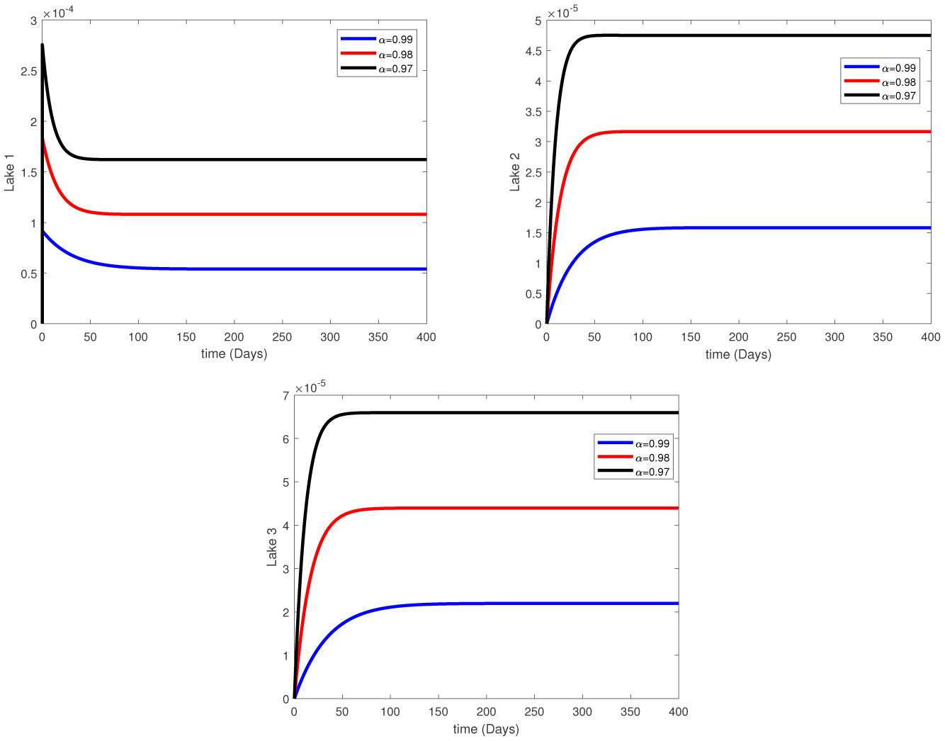
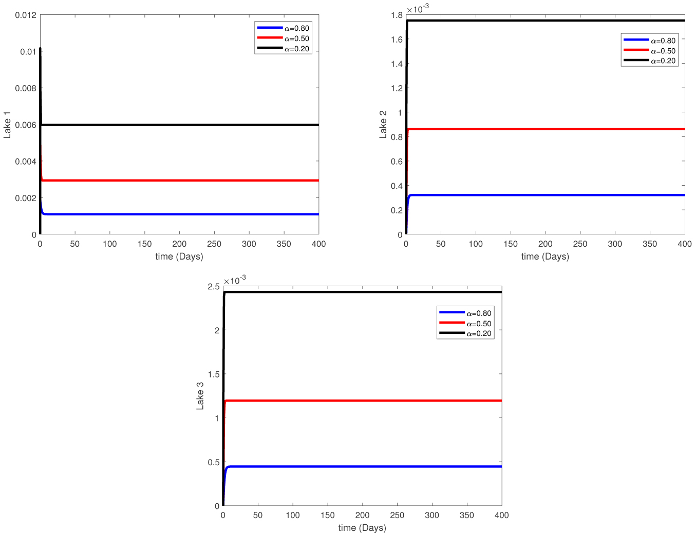
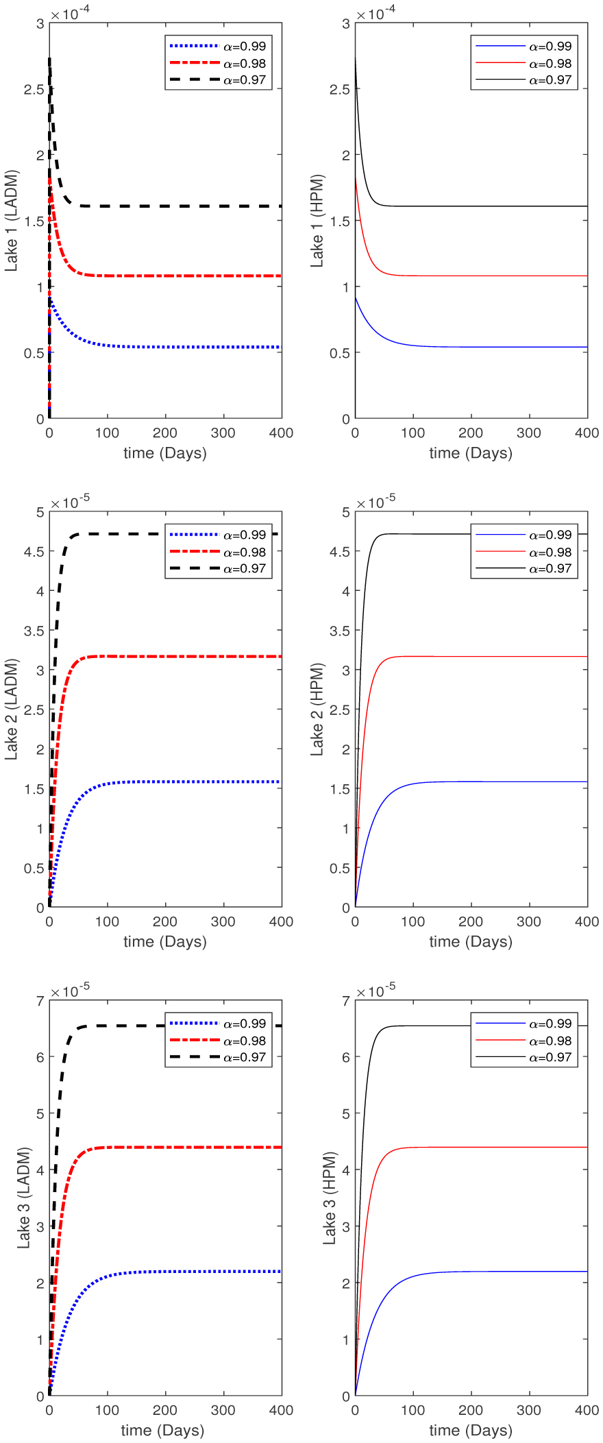
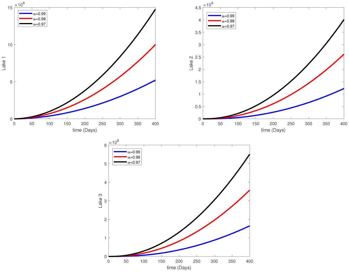
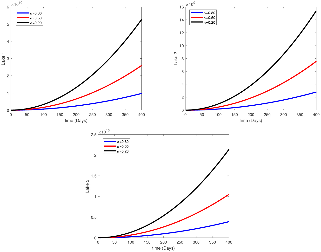
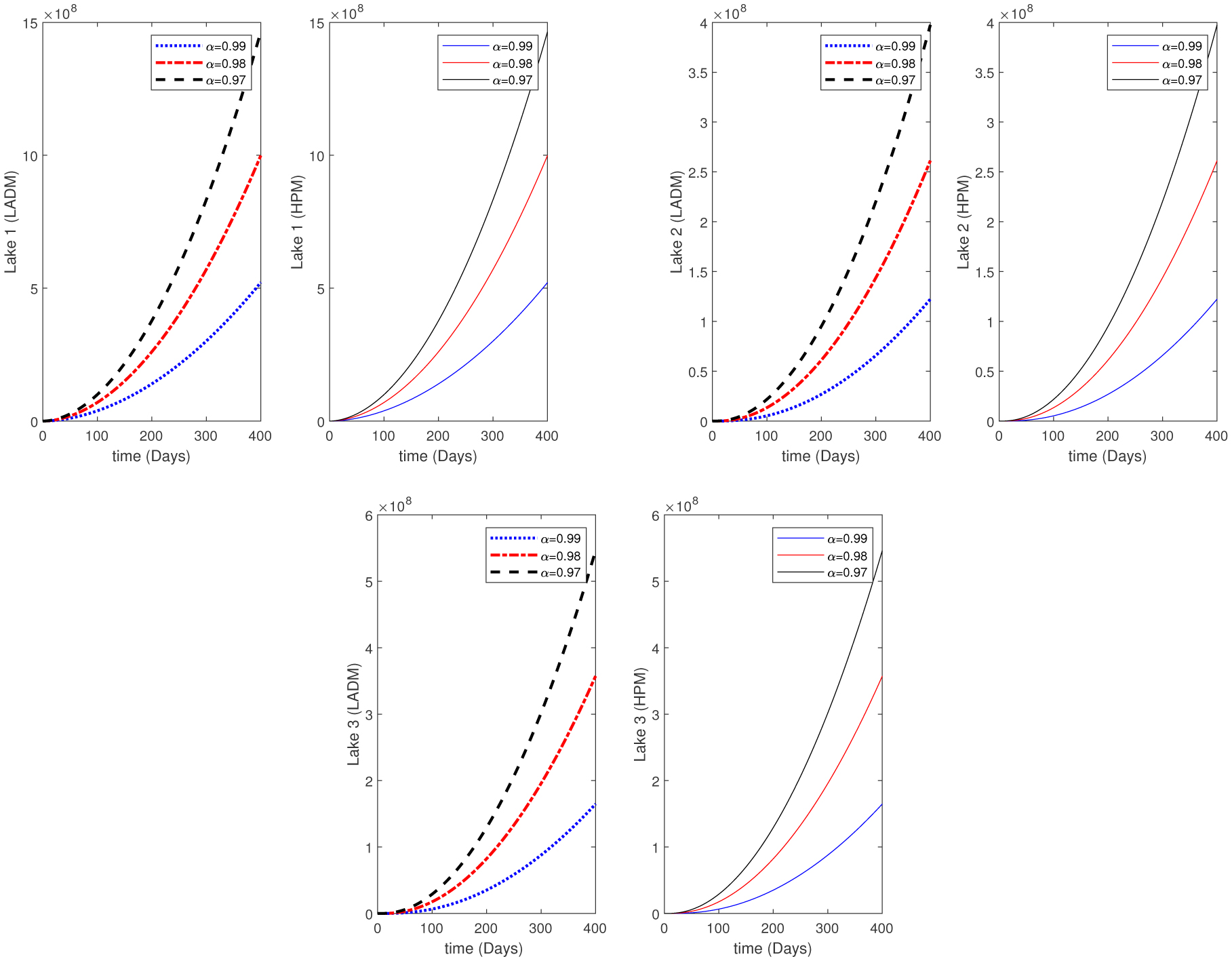
Water pollution is a critical global concern that demands ongoing scrutiny and revision of water resource policies at all levels to safeguard a healthy living environment. In this study, we focus on examining the dynamics of a fractional-order model involving three interconnected lakes, utilizing the Caputo differential operator. The aim is to investigate the issue of lake pollution by analyzing a system of linear equations that represent the interconnecting waterways. To numerically solve the model, we employ two methods: The Laplace transform with the Adomian decomposition method (LADM) and the Homotopy perturbation method (HPM). We compare the obtained numerical solutions from both methods and present the results. The study encompasses three variations of the model: the periodic input model, the exponentially decaying input model, and the linear input model. MATLAB is employed to conduct numerical simulations for the proposed scheme, considering various fractional orders. The numerical results are further supported by informative graphical illustrations. Through simulation, we validate the suitability of the proposed model for addressing the issue at hand. The outcomes of this research contribute to the understanding and management of water pollution, aiding policymakers and researchers in formulating effective strategies for maintaining water quality and protecting our environment.

Keywords:

Citation: Yasir Nadeem Anjam, Mehmet Yavuz, Mati ur Rahman, Amna Batool. Analysis of a fractional pollution model in a system of three interconnecting lakes[J]. AIMS Biophysics, 2023, 10(2): 220-240. doi: 10.3934/biophy.2023014

Related Papers:

[1]	Mati ur Rahman, Mehmet Yavuz, Muhammad Arfan, Adnan Sami . Theoretical and numerical investigation of a modified ABC fractional operator for the spread of polio under the effect of vaccination. AIMS Biophysics, 2024, 11(1): 97-120. doi: 10.3934/biophy.2024007
[2]	Shaimaa A. M. Abdelmohsen, D. Sh. Mohamed, Haifa A. Alyousef, M. R. Gorji, Amr M. S. Mahdy . Mathematical modeling for solving fractional model cancer bosom malignant growth. AIMS Biophysics, 2023, 10(3): 263-280. doi: 10.3934/biophy.2023018
[3]	Mohammed Alabedalhadi, Mohammed Shqair, Ibrahim Saleh . Analysis and analytical simulation for a biophysical fractional diffusive cancer model with virotherapy using the Caputo operator. AIMS Biophysics, 2023, 10(4): 503-522. doi: 10.3934/biophy.2023028
[4]	Ken Takahashi, Takayuki Oda, Keiji Naruse . Coarse-grained molecular dynamics simulations of biomolecules. AIMS Biophysics, 2014, 1(1): 1-15. doi: 10.3934/biophy.2014.1.1
[5]	Nor Afiqah Mohd Aris, Siti Suhana Jamaian . Dynamical analysis of fractional-order chemostat model. AIMS Biophysics, 2021, 8(2): 182-197. doi: 10.3934/biophy.2021014
[6]	Alexander Galashev . Computer implementation of the method for electrolytic production of thin films for biomedical applications: short review. AIMS Biophysics, 2024, 11(1): 39-65. doi: 10.3934/biophy.2024004
[7]	Soumaya Eltifi-Ghanmi, Samiha Amara, Bessem Mkaouer . Kinetic and kinematic analysis of three kicks in Sanda Wushu. AIMS Biophysics, 2025, 12(2): 174-196. doi: 10.3934/biophy.2025011
[8]	Mehmet Yavuz, Fuat Usta . Importance of modelling and simulation in biophysical applications. AIMS Biophysics, 2023, 10(3): 258-262. doi: 10.3934/biophy.2023017
[9]	Carlo Bianca . Mathematical and computational modeling of biological systems: advances and perspectives. AIMS Biophysics, 2021, 8(4): 318-321. doi: 10.3934/biophy.2021025
[10]	Julia C. Arciero, Paola Causin, Francesca Malgaroli . Mathematical methods for modeling the microcirculation. AIMS Biophysics, 2017, 4(3): 362-399. doi: 10.3934/biophy.2017.3.362

Abstract

1. Introduction

In line with the Environmental Health Association of America's committee definition, the environment encompasses the habitats where humans reside, work, and engage in recreational activities. It includes the air we breathe, the food we consume, the water we drink, and the shelter we seek for protection against the elements. Additionally, it comprises harmful pollutants and other environmental factors that significantly impact our well-being and overall health. Our survival depends on access to nutritious food, clean air, and safe drinking water, which necessitates the promotion of a healthy atmosphere. The World Health Organization (WHO) emphasizes the importance of maintaining a clean environment that adheres to health standards. Regrettably, our water supply has become increasingly contaminated, with numerous pollutants affecting the quality of our drinking water sources. Thus, it is imperative that we develop a conscientious awareness of our surroundings. Environmental science encompasses scientific methodologies, economic considerations, and political interventions. Moreover, toxic substances introduced into lakes, streams, rivers, seas, and other bodies of water can dissolve, remain suspended, or settle at the bottom. Consequently, water contamination ensues, leading to a decline in groundwater quality and the deterioration of marine habitats [1].

Pollution can also seep into the groundwater and alter the sediment composition. Water pollution has various causes, with sewage and industrial waste being the most significant contributors that enter rivers. In many developed countries, the resources allocated for waste management are insufficient [2]. Currently, only around 10% of the generated wastewater is properly treated, while the rest is discharged and deposited into our water bodies. Consequently, impurities infiltrate groundwater, tributaries, and other water sources. The water that ultimately reaches our homes is often highly contaminated, carrying viruses that can harm microorganisms. Another major source of water pollution is agricultural runoff, which involves the drainage of water from fields containing pesticides and fertilizers. Domestic sewage, also known as sanitary sewage, refers to wastewater discharged from households. This type of water contains a wide array of dissolved and suspended contaminants.

Mathematical frameworks play a crucial role in predicting and addressing social issues, and they have been increasingly utilized in recent decades to mitigate the impact of these issues. By applying mathematical models, we can effectively control the spread of real-world problems. As many global challenges exhibit quasi-linear characteristics, relying solely on linear models can often lead to idealistic and unrealistic outcomes. Therefore, non-linear mathematical models provide a more accurate depiction of real-world issues. In the context of modeling lake contamination, a collocation approach has been proposed, which utilizes Bessel polynomials and collocation points to generate an updated matrix problem [3]. This approach allows for a more comprehensive understanding of the contamination dynamics within a lake system. Additionally, the homotopy perturbation approach has been employed to offer approximate and analytical solutions for nonlinear ordinary differential equation systems, such as those encountered in modeling lake contamination [4]. Furthermore, the differential transform method (DTM) has been utilized to analyze pollution models involving interconnected systems of three lakes connected by waterways [5]. These mathematical methods enhance our ability to study and address the complex dynamics of pollution in various environmental systems.

A fractional differential equation system has been investigated by Haq EU [6]. He designed the system to simulate the pollution of a group of lakes and assess the results using other well-known analytical approaches, such as iterative variation and Adomian decomposition. The Laplace Adomian decomposition method is widely applied to solve many real-life problems (see [7]–[9]). Several researchers have used the technique of LADM to investigate different types of problems. For example, in [10], the authors examined the free vibrations of a non-uniform Bernoulli beam using LADM. In [11], a fractional-order sterile insect technology model was studied with the help of LADM. Other studies include the investigation of MHD flow of incompressible fluid between two parallel plates [12], and the study of the effect of a magnetic field on the heat transfer of carbon nanotubes [13]. Different approaches have been used for disease models, studying them with various fractional operator techniques [14]–[23].

Aguirre and Tully [24] employed simple mixture problem methodologies to develop a differential equation that characterizes the pollution concentration in a lake. Prakasha and Veeresha [25] explored three alternative scenarios of the model and established an approximate analytical solution for the system of three fractional differential equations using the q-homotopy analysis transform technique (q-HATM). The results obtained demonstrated the high effectiveness and systematic nature of the proposed strategy. Khalid and Sultana [26] utilized the perturbation-iteration approach to estimate the solution of three input models: periodic, linear step, and exponentially decaying. As a reference, the analytical simulation of the lake system problem was conducted using the fourth-order Runge-Kutta technique (RK4). Biazar and Farrokhi [27] employed compartmental modeling to predict the contamination of a system of lakes through a set of mathematically-researched equations. Bazar and Shahbala [28] utilized the variational iteration method (VIM), and the results demonstrated that the variational iteration approach was easier to implement compared to the Adomian decomposition method for pollution monitoring in lakes. Three distinct types of input models were considered: sinusoidal, impulse, and step. Furthermore, Toufik and Atangana's novel numerical technique was applied [29] to examine the updated model of the contaminated lake system.

Fractional calculus, despite its name, deals with integrals and derivatives of any positive real order and can be considered a branch of mathematical modeling. It focuses on integrodifferential operators and equations with convolution-type integrals that involve weakly singular kernels of power-law form. It is closely related to the theory of pseudo-differential operators. In recent years, fractional calculus has garnered significant attention from researchers, and various aspects of this subject are being explored in research [30], [31]. This is because fractional derivatives serve as an important tool for describing the dynamic behavior of diverse physical systems [32]–[34]. The distinct characteristic of these differential operators lies in their non-local nature, which is absent in integer-order differential operators [35]. In fact, fractional order models are more accurate and practical than classical integer order models, and techniques such as the Legendre operational matrix can be extended to incorporate fractional calculus [36], [37]. The application of fractional differential equations in applied sciences is another area of interest [38], [39].

Fractional order derivatives offer increased flexibility in modeling various biomaterials and systems [40]. They provide powerful tools for characterizing the dynamic behavior of these systems. There are different types of fractional derivatives, such as Riemann and Liouville, and Caputo operators, which are commonly used in practice. Caputo [41] introduced a fractional derivative that allows for the incorporation of conventional initial and boundary conditions relevant to real-world problems. While these fractional derivatives offer improved accuracy in describing real phenomena compared to integer-order derivatives, their kernel functions may result in singularities that lead to computational challenges. To explore fractional mathematical models beyond the traditional Caputo derivative, various methodologies, including iterative and numerical methods, have been employed [42]–[44]. In this study, we focus on a system of three equations that describes lake contamination. The model represents the contamination of a three-lake system [27], as illustrated in Figure 1.

Figure 1. System of three lakes with interconnecting channels.

DownLoad: Full-Size Img PowerPoint

The arrows in the figure indicate the direction of flow in the channels or pipes. In this system, a contaminant is introduced into the first lake through a factory, and the rate of entrance of the pollutant into the lake per unit of time is represented by the function p(t). The function p(t) can be constant or vary over time. The goal is to determine the level of pollution in each lake at any given time. At time t ≥ 0, the contamination level c_i(t) in Lake i is proportional to the volume of water v_i and the concentration of pollutant y_i(t) in the following manner:

$c_{i} (t) = \frac{y_{i} (t)}{v_{i}} .$

In the lake system, it is assumed that each lake is initially free of any contaminants, so the concentration of pollutant in each lake at time t = 0 is given by y_i(0) = 0 for i = 1, 2, 3. To simulate the dynamic behavior of the lake system, a constant g_ji is used to represent the flow rate from lake i to lake j. The flux of pollutant flowing from lake i into lake j at any time t is denoted by r_ji(t) and is defined as follows:

$r_{j i} (t) = g_{j i} c_{i} (t) = \frac{g_{j i}}{v_{i}} y_{i} (t) .$

Thus, r_ji(t) represents the proportion at which the contamination level in lake i flows into lake j at time t. It is important to note this relationship.

Rate of change of pollutant = Input rate - Output rate.

Applying this principle to each lake, we obtain the following system of differential equations:

$(\begin{matrix} \frac{d y_{1}}{d t} = \frac{g_{13}}{v_{3}} y_{3} (t) + p (t) - \frac{g_{31}}{v_{1}} y_{1} (t) - \frac{g_{21}}{v_{1}} y_{1} (t), \\ \frac{d y_{2}}{d t} = \frac{g_{21}}{v_{1}} y_{1} (t) - \frac{g_{32}}{v_{2}} y_{2} (t), \\ \frac{d y_{3}}{d t} = \frac{g_{31}}{v_{1}} y_{1} (t) + \frac{g_{32}}{v_{2}} y_{2} (t) - \frac{g_{13}}{v_{3}} y_{3} (t) . \end{matrix}$ (1.1)

It is apparent from this that the incoming and outgoing flow rates in each lake are constant, and as a result, the water volume in each lake remains fixed. Therefore, we can establish the following conditions:

$(\begin{matrix} L a k e 1 : g_{13} = g_{21} + g_{31}, \\ L a k e 2 : g_{21} = g_{32}, \\ L a k e 3 : g_{31} + g_{32} = g_{13} . \end{matrix}$

To evaluate the performance of the proposed model, we consider specific predicted values as listed in [27], which can be expressed as follows:

$g_{21} = g_{32} = 18 m i^{3} / y e a r, g_{31} = 20 m i^{3} / y e a r, g_{13} = 38 m i^{3} / y e a r, v_{1} = 2900 m i^{3}, v_{2} = 850 m i^{3}, v_{3} = 1180 m i^{3} .$

In this study, to obtain a more accurate qualitative and numerical iterative analysis of the proposed model, we consider the system (1.1) in terms of the Caputo fractional order differential operator. The system can be expressed as follows:

$(\begin{matrix} ^{c} D_{t}^{α} y_{1} (t) = \frac{g_{13}^{α}}{v_{3}^{α}} y_{3} (t) + p (t) - \frac{g_{31}^{α}}{v_{1}^{α}} y_{1} (t) - \frac{g_{21}^{α}}{v_{1}^{α}} y_{1} (t), \\ ^{c} D_{t}^{α} y_{2} (t) = \frac{g_{21}^{α}}{v_{1}^{α}} y_{1} (t) - \frac{g_{32}^{α}}{v_{2}^{α}} y_{2} (t), \\ ^{c} D_{t}^{α} y_{3} (t) = \frac{g_{31}^{α}}{v_{1}^{α}} y_{1} (t) + \frac{g_{32}^{α}}{v_{2}^{α}} y_{2} (t) - \frac{g_{13}^{α}}{v_{3}^{α}} y_{3} (t), \end{matrix}$ (1.2)

where α denotes the fractional order.

The objective of this study is to analyze a system of fractional differential equations that describe lake pollution and provide meaningful insights through a mathematical model that can explain real-world scenarios using a simple and efficient approach. It is important to highlight that the investigated model heavily relies on time and its history, which can be systematically incorporated and represented using the newly developed fractional operator. To obtain the solution of the model, we utilize the Laplace transform in conjunction with the Adomian decomposition method and the Homotopy perturbation method. These techniques enable us to obtain an approximate solution for the considered model. Additionally, we compare the results obtained from both techniques, demonstrating their identical nature. Furthermore, we employ MATLAB to facilitate the numerical solutions and depict the pollution levels in each lake graphically, considering arbitrary fractional orders. This visual representation aids in understanding the behavior of the lake system under different scenarios.

The structure of this paper is organized as follows: Section 2 provides fundamental results and definitions related to the topic. In Section 3, the general solutions of the suggested model are obtained using the Laplace Adomian decomposition technique. This section focuses on the qualitative analysis of the model. Section 4 presents the general solutions of the considered model using the Homotopy perturbation technique. This section discusses the application of the Homotopy perturbation method for obtaining the solutions. In Section 5, a graphical comparison of the numerical solutions obtained from both the Laplace Adomian decomposition technique and the Homotopy perturbation technique is presented. The numerical simulation results are briefly discussed in this section. Finally, in Section 6, the concluding remarks of the study are provided.

2. Preliminaries and basic definitions

In this section, some essential preliminaries and fractional calculus results are presented in line with [45], [46].

Definition 2.1. For α > 0 with $n - 1 < α < n$ , $n \in ℕ$ , the Caputo fractional order derivative of the function f(x) is described as follows:

$^{c} D_{x}^{α} f (x) = \frac{d^{α}}{d t^{α}} f (t) = \frac{1}{Γ (n - α)} \int_{0}^{x} {(x - t)}^{n - α - 1} \frac{d^{n}}{d t^{n}} f (t) d t,$

such that the integral part on the right exists and n = [α] + 1, and the symbol Γ denotes the Gamma function which is described as

$Γ (n) = \int_{0}^{\infty} e^{- t} t^{n - 1} d t .$

Definition 2.2. The Laplace transform of g(t) in the general framework of Caputo definition is described as follows:

$ℒ [^{c} D_{t}^{α} g (t)] = s^{α} G (s) - \sum_{j = 0}^{m - 1} s^{α - j - 1} g^{k} (0), m - 1 < α, m \in ℕ .$

Definition 2.3. The Homotopy perturbation method (HPM) is a semi-analytical technique used to solve linear and nonlinear ordinary and partial differential equations, as well as systems of equations. It is also applicable to systems consisting of both linear and nonlinear differential equations. One notable advantage of using the HPM over decomposition methods is that it can handle nonlinear problems without requiring the use of Adomian polynomials. The HPM was first proposed by the Chinese mathematician He [47], who introduced the concept of forming a homotopy $ν (l, p) : Ω \times [0,1] \to ℝ$ for an equation involving both linear and nonlinear components.

$F (ν, p) = (1 - p) [L (ν) - L (u_{0})] + p [L (ν) + N (ν) - f (l)] = 0,$

where L is used for the linear part, N for the nonlinear part, l ∈ Ω, Ω is a topological space and p ∈ [0,1] is the embedding parameter. Furthermore, u₀ is an initial approximation that satisfies the boundary conditions.

3. General solution of the model (1.2) by (LADM)

In this section, we will discuss the general technique of the Laplace Adomian decomposition method (LADM) to construct the solution for the considered model (1.2), along with the initial conditions. We will also demonstrate how to integrate the LADM with the Caputo differential operator.

$(\begin{matrix} ^{c} D_{t}^{α} y_{1} (t) = \frac{g_{13}}{v_{3}} y_{3} (t) + p (t) - \frac{g_{31}}{v_{1}} y_{1} (t) - \frac{g_{21}}{v_{1}} y_{1} (t), \\ ^{c} D_{t}^{α} y_{2} (t) = \frac{g_{21}}{v_{1}} y_{1} (t) - \frac{g_{32}}{v_{2}} y_{2} (t), \\ ^{c} D_{t}^{α} y_{3} (t) = \frac{g_{31}}{v_{1}} y_{1} (t) + \frac{g_{32}}{v_{2}} y_{2} (t) - \frac{g_{13}}{v_{3}} y_{3} (t), \end{matrix}$ (3.1)

with subject to the initial conditions:

$y_{1} (0) = n_{1}, y_{2} (0) = n_{2}, y_{3} (0) = n_{3} .$

Now, taking the Laplace transform of (3.1) in the Caputo sense, one may get

$(\begin{matrix} ℒ [^{c} D_{t}^{α} y_{1} (t)] = ℒ [\frac{g_{13}}{v_{3}} y_{3} (t) + p (t) - \frac{g_{31}}{v_{1}} y_{1} (t) - \frac{g_{21}}{v_{1}} y_{1} (t)], \\ ℒ [^{c} D_{t}^{α} y_{2} (t)] = ℒ [\frac{g_{21}}{v_{1}} y_{1} (t) - \frac{g_{32}}{v_{2}} y_{2} (t)], \\ ℒ [^{c} D_{t}^{α} y_{3} (t)] = ℒ [\frac{g_{31}}{v_{1}} y_{1} (t) + \frac{g_{32}}{v_{2}} y_{2} (t) - \frac{g_{13}}{v_{3}} y_{3} (t)], \end{matrix}$ (3.2)

using the initial conditions yields

$(\begin{matrix} ℒ [y_{1} (t)] = \frac{n_{1}}{s} + \frac{1}{s^{α}} ℒ [\frac{g_{13}}{v_{3}} y_{3} (t) + p (t) - \frac{g_{31}}{v_{1}} y_{1} (t) - \frac{g_{21}}{v_{1}} y_{1} (t)], \\ ℒ [y_{2} (t)] = \frac{n_{2}}{s} + \frac{1}{s^{α}} ℒ [\frac{g_{21}}{v_{1}} y_{1} (t) - \frac{g_{32}}{v_{2}} y_{2} (t)], \\ ℒ [y_{3} (t)] = \frac{n_{3}}{s} + \frac{1}{s^{α}} ℒ [\frac{g_{31}}{v_{1}} y_{1} (t) + \frac{g_{32}}{v_{2}} y_{2} (t) - \frac{g_{13}}{v_{3}} y_{3} (t)] . \end{matrix}$ (3.3)

Assuming the solution for y₁(t), y₂(t) and y₃(t) in an infinite series is given below:

$\begin{matrix} (\begin{matrix} y_{1} (t) = \sum_{n = 0}^{\infty} y_{1 (n)} (t), \\ y_{2} (t) = \sum_{n = 0}^{\infty} y_{2 (n)} (t), \\ y_{3} (t) = \sum_{n = 0}^{\infty} y_{3 (n)} (t), \end{matrix} \end{matrix}$

using the above series in (3.3), and comparing like terms on both sides, one can get

$(\begin{matrix} ℒ [y_{1 (0)} (t)] = \frac{n_{1}}{s}, ℒ [y_{2 (0)} (t)] = \frac{n_{2}}{s}, ℒ [y_{3 (0)} (t)] = \frac{n_{3}}{s}, \\ ℒ [y_{1 (1)} (t)] = \frac{1}{s^{α}} ℒ [\frac{g_{13}}{v_{3}} y_{3 (0)} (t) + p (t) - \frac{g_{31}}{v_{1}} y_{1 (0)} (t) - \frac{g_{21}}{v_{1}} y_{1 (0)} (t)], \\ ℒ [y_{2 (1)} (t)] = \frac{1}{s^{α}} ℒ [\frac{g_{21}}{v_{1}} y_{1 (0)} (t) - \frac{g_{32}}{v_{2}} y_{2 (0)} (t)], \\ ℒ [y_{3 (1)} (t)] = \frac{1}{s^{α}} ℒ [\frac{g_{31}}{v_{1}} y_{1 (0)} (t) + \frac{g_{32}}{v_{2}} y_{2 (0)} (t) - \frac{g_{13}}{v_{3}} y_{3 (0)} (t)], \\ ⋮ \\ ℒ [y_{1 (n + 1)} (t)] = \frac{1}{s^{α}} ℒ [\frac{g_{13}}{v_{3}} y_{3 (n)} (t) + p (t) - \frac{g_{31}}{v_{1}} y_{1 (n)} (t) - \frac{g_{21}}{v_{1}} y_{1 (n)} (t)], \\ ℒ [y_{2 (n + 1)} (t)] = \frac{1}{s^{α}} ℒ [\frac{g_{21}}{v_{1}} y_{1 (n)} (t) - \frac{g_{32}}{v_{2}} y_{2 (n)} (t)], \\ ℒ [y_{3 (n + 1)} (t)] = \frac{1}{s^{α}} ℒ [\frac{g_{31}}{v_{1}} y_{1 (n)} (t) + \frac{g_{32}}{v_{2}} y_{2 (n)} (t) - \frac{g_{13}}{v_{3}} y_{3 (n)} (t)] . \end{matrix}$ (3.4)

Further, utilizing the inverse Laplace transform to equation (3.4), we have

$(\begin{matrix} y_{1 (0)} (t) = n_{1}, y_{2 (0)} (t) = n_{2}, y_{3 (0)} (t) = n_{3}, \\ y_{1 (1)} (t) = [\frac{g_{13}}{v_{3}} n_{3} + p (t) - \frac{g_{31}}{v_{1}} n_{1} - \frac{g_{21}}{v_{1}} n_{1}] \frac{t^{α}}{Γ (α + 1)}, \\ y_{2 (1)} (t) = [\frac{g_{21}}{v_{1}} n_{1} - \frac{g_{32}}{v_{2}} n_{2}] \frac{t^{α}}{Γ (α + 1)}, \\ y_{3 (1)} (t) = [\frac{g_{31}}{v_{1}} n_{1} + \frac{g_{32}}{v_{2}} n_{2} - \frac{g_{13}}{v_{3}} n_{3}] \frac{t^{α}}{Γ (α + 1)}, \\ y_{1 (2)} (t) = [\frac{g_{13}}{v_{3}} x_{11} + p (t) - \frac{g_{31}}{v_{1}} w_{11} - \frac{g_{21}}{v_{1}} w_{11}] \frac{t^{2 α}}{Γ (2 α + 1)}, \\ y_{2 (2)} (t) = [\frac{g_{21}}{v_{1}} w_{11} - \frac{g_{32}}{v_{2}} u_{11}] \frac{t^{2 α}}{Γ (2 α + 1)}, \\ y_{3 (2)} (t) = [\frac{g_{31}}{v_{1}} w_{11} + \frac{g_{32}}{v_{2}} u_{11} - \frac{g_{13}}{v_{3}} x_{11}] \frac{t^{2 α}}{Γ (2 α + 1)}, \\ y_{1 (3)} (t) = [\frac{g_{13}}{v_{3}} x_{111} + p (t) - \frac{g_{31}}{v_{1}} w_{111} - \frac{g_{21}}{v_{1}} w_{111}] \frac{t^{3 α}}{Γ (3 α + 1)}, \\ y_{2 (3)} (t) = [\frac{g_{21}}{v_{1}} w_{111} - \frac{g_{32}}{v_{2}} u_{111}] \frac{t^{3 α}}{Γ (3 α + 1)}, \\ y_{3 (3)} (t) = [\frac{g_{31}}{v_{1}} w_{111} + \frac{g_{32}}{v_{2}} u_{111} - \frac{g_{13}}{v_{3}} x_{111}] \frac{t^{3 α}}{Γ (3 α + 1)} . \end{matrix}$

Additionally, the remaining terms can be derived in a similar fashion. The unknown values in the aforementioned equations are listed below:

$(\begin{matrix} w_{11} = \frac{g_{13}}{v_{3}} n_{3} + p (t) - \frac{g_{31}}{v_{1}} n_{1} - \frac{g_{21}}{v_{1}} n_{1}, \\ u_{11} = \frac{g_{21}}{v_{1}} n_{1} - \frac{g_{32}}{v_{2}} n_{2}, \\ x_{11} = \frac{g_{31}}{v_{1}} n_{1} + \frac{g_{32}}{v_{2}} n_{2} - \frac{g_{13}}{v_{3}} n_{3}, \\ w_{111} = \frac{g_{13}}{v_{3}} x_{11} + p (t) - \frac{g_{31}}{v_{1}} w_{11} - \frac{g_{21}}{v_{1}} w_{11}, \\ u_{111} = \frac{g_{21}}{v_{1}} w_{11} - \frac{g_{32}}{v_{2}} u_{11}, \\ x_{111} = \frac{g_{31}}{v_{1}} w_{11} + \frac{g_{32}}{v_{2}} u_{11} - \frac{g_{13}}{v_{3}} x_{11} . \end{matrix}$

4. General solution for model (1.2) with (HPM)

We will now apply the Homotopy Perturbation Method (HPM) to derive the general solution of Model (1.2) as:

$(\begin{matrix} (1 - q {) [}^{c} D_{t}^{α} (y_{1} (t)) -^{c} D_{t}^{α} (y_{1 (0)} (t))] + q [^{c} D_{t}^{α} (y_{1} (t)) - \frac{g_{13}}{v_{3}} y_{3} (t) - p (t) + \frac{g_{31}}{v_{1}} y_{1} (t) + \frac{g_{21}}{v_{1}} y_{1} (t)] = 0, \\ (1 - q {) [}^{c} D_{t}^{α} (y_{2} (t)) -^{c} D_{t}^{α} (y_{2 (0)} (t))] + q [^{c} D_{t}^{α} (y_{2} (t)) - \frac{g_{21}}{v_{1}} y_{1} (t) + \frac{g_{32}}{v_{2}} y_{2} (t)] = 0, \\ (1 - q {) [}^{c} D_{t}^{α} (y_{3} (t)) -^{c} D_{t}^{α} (y_{3 (0)} (t))] + q [^{c} D_{t}^{α} (y_{3} (t)) - \frac{g_{31}}{v_{1}} y_{1} (t) - \frac{g_{32}}{v_{2}} y_{2} (t) + \frac{g_{13}}{v_{3}} y_{3} (t)] = 0. \end{matrix}$ (4.1)

By substituting q = 0 into equation (4.1), we obtain the following system of fractional differential equations:

$(\begin{matrix} ^{c} D_{t}^{α} (y_{1} (t)) -^{c} D_{t}^{α} (y_{1 (0)} (t)) = 0, \\ ^{c} D_{t}^{α} (y_{2} (t)) -^{c} D_{t}^{α} (y_{2 (0)} (t)) = 0, \\ ^{c} D_{t}^{α} (y_{3} (t)) -^{c} D_{t}^{α} (y_{3 (0)} (t)) = 0. \end{matrix}$ (4.2)

The solution to the above equation is straightforward. Next, setting q = 1 in equation (4.1) results in a similar model to equation (1.2). We assume the solution takes the form of an infinite series as:

$(\begin{matrix} y_{1} (t) = \sum_{n = 0}^{\infty} q^{n} y_{1 (n)} (t), \\ y_{2} (t) = \sum_{n = 0}^{\infty} q^{n} y_{2 (n)} (t), \\ y_{3} (t) = \sum_{n = 0}^{\infty} q^{n} y_{3 (n)} (t) . \end{matrix}$ (4.3)

Furthermore, the original system can be obtained by substituting q = 1 into equation (4.1). By substituting equation (4.3) into equation (4.1) and comparing the terms with respect to the powers of q, we obtain:

$q^{0} : (\begin{matrix} y_{1 (0)} (t) = y_{1} (0) = n_{1}, \\ y_{2 (0)} (t) = y_{2} (0) = n_{2}, \\ y_{3 (0)} (t) = y_{3} (0) = n_{3} . \end{matrix}$ (4.4)

Similarly,

$q^{1} : (\begin{matrix} y_{1 (1)} (t) = [\frac{g_{13}}{v_{3}} n_{3} + p (t) - \frac{g_{31}}{v_{1}} n_{1} - \frac{g_{21}}{v_{1}} n_{1}] \frac{t^{α}}{Γ (α + 1)}, \\ y_{2 (1)} (t) = [\frac{g_{21}}{v_{1}} n_{1} - \frac{g_{32}}{v_{2}} n_{2}] \frac{t^{α}}{Γ (α + 1)}, \\ y_{3 (1)} (t) = [\frac{g_{31}}{v_{1}} n_{1} + \frac{g_{32}}{v_{2}} n_{2} - \frac{g_{13}}{v_{3}} n_{3}] \frac{t^{α}}{Γ (α + 1)} . \end{matrix}$ (4.5)

$q^{2} : (\begin{matrix} y_{1 (2)} (t) = [\frac{g_{13}}{v_{3}} x_{11} + p (t) - \frac{g_{31}}{v_{1}} w_{11} - \frac{g_{21}}{v_{1}} w_{11}] \frac{t^{2 α}}{Γ (2 α + 1)}, \\ y_{2 (2)} (t) = [\frac{g_{21}}{v_{1}} w_{11} - \frac{g_{32}}{v_{2}} u_{11}] \frac{t^{2 α}}{Γ (2 α + 1)}, \\ y_{3 (2)} (t) = [\frac{g_{31}}{v_{1}} w_{11} + \frac{g_{32}}{v_{2}} u_{11} - \frac{g_{13}}{v_{3}} x_{11}] \frac{t^{2 α}}{Γ (2 α + 1)} . \end{matrix}$ (4.6)

The approximate series solution is thus acquired. In the next section, we will do simulation for the aforementioned methods.

5. Numerical results and simulations

In this section, we conduct numerical simulations to complement the analytical findings of our proposed model. The simulations involve qualitative point analysis and consider the parameters from a biological feasibility perspective. By using the parametric values, we determine the following terms of the proposed model:

$(\begin{matrix} y_{1 (0)} (t) = 0, y_{2 (0)} (t) = 0, y_{3 (0)} (t) = 0, \\ y_{1 (1)} (t) = p (t) \frac{t^{α}}{Γ (α + 1)}, y_{2 (1)} (t) = 0, y_{3 (1)} (t) = 0, \\ y_{1 (2)} (t) = (0.999) p (t) \frac{t^{2 α}}{Γ (2 α + 1)}, y_{2 (2)} (t) = (0.006206) p (t) \frac{t^{2 α}}{Γ (2 α + 1)}, \\ y_{3 (2)} (t) = (0.00689) p (t) \frac{t^{2 α}}{Γ (2 α + 1)}, \\ y_{1 (3)} (t) = (0.98713) p (t) \frac{t^{3 α}}{Γ (3 α + 1)}, \\ y_{2 (3)} (t) = (0.006069) p (t) \frac{t^{3 α}}{Γ (3 α + 1)}, \\ y_{3 (3)} (t) = (0.00679) p (t) \frac{t^{3 α}}{Γ (3 α + 1)} . \end{matrix}$ (5.1)

Furthermore, the solutions to the first few terms are given as:

$(\begin{matrix} y_{1} (t) = p (t) \frac{t^{α}}{Γ (α + 1)} + (0.999) p (t) \frac{t^{2 α}}{Γ (2 α + 1)} + (0.98713) p (t) \frac{t^{3 α}}{Γ (3 α + 1)}, \\ y_{2} (t) = (0.006206) p (t) \frac{t^{2 α}}{Γ (2 α + 1)} + (0.006069) p (t) \frac{t^{3 α}}{Γ (3 α + 1)}, \\ y_{3} (t) = (0.00689) p (t) \frac{t^{2 α}}{Γ (2 α + 1)} + (0.00679) p (t) \frac{t^{3 α}}{Γ (3 α + 1)} . \end{matrix}$ (5.2)

Now, evaluating (5.2) for α = 0.97, one get

$(\begin{matrix} y_{1} (t) = 1.012468567 p (t) t^{0.97} + 0.5275576582 p (t) t^{1.94} + 0.1839995904 p (t) t^{2.91}, \\ y_{2} (t) = 0.006283379927 p (t) t^{1.94} + 0.003204952380 p (t) t^{2.91}, \\ y_{3} (t) = 0.006975908427 p (t) t^{1.94} + 0.003585702201 p (t) t^{2.91} . \end{matrix}$ (5.3)

Similarly, for α = 0.98, the approximations are:

$(\begin{matrix} y_{1} (t) = 1.008360917 p (t) t^{0.98} + 0.5181171462 p (t) t^{1.96} + 0.1773092790 p (t) t^{2.94}, \\ y_{2} (t) = 0.006257887851 p (t) t^{1.96} + 0.003147600561 p (t) t^{2.94}, \\ y_{3} (t) = 0.006947606718 p (t) t^{1.96} + 0.003521536960 p (t) t^{2.94} . \end{matrix}$ (5.4)

And for α = 0.99, one can obtain the approximate solutions are:

$(\begin{matrix} y_{1} (t) = 1.004204343 p (t) t^{0.99} + 0.5087639171 p (t) t^{1.98} + 0.1708178394 p (t) t^{2.97}, \\ y_{2} (t) = 0.006232092153 p (t) t^{1.98} + 0.003090778992 p (t) t^{2.97}, \\ y_{3} (t) = 0.006918967923 p (t) t^{1.98} + 0.003457964962 p (t) t^{2.97} . \end{matrix}$ (5.5)

Furthermore, we have considered three different types of input functions to represent the duration of the contaminant in each lake. These input functions include periodic, exponentially decaying, and linear inputs.

Case 1: Periodic Input Model: In this scenario, the model is evaluated when pollution is periodically introduced into Lake 1. We have chosen the input function $p (t) = a s i n (ω t) + c$ , where a and ω represent the amplitude and frequency of the fluctuations, respectively, and c represents the average pollutant concentration input. For this example, let us consider a = ω = c = 1 as an illustration. This could represent a manufacturing facility that discharges waste during the day and generates more pollutants during the night due to increased production during that time. As a result, the pollutant input exhibits a periodic pattern. By applying this periodic input to the model, the concentration levels in the lakes eventually converge to the average input level of the contaminant.

Figure 2. Adaptive nature of the approximated LADM solutions for y₁, y₂, and y₃ at different arbitrary fractional orders for the Case 1.

DownLoad: Full-Size Img PowerPoint

Figure 3. Dynamical behavior of the considered model with LADM solutions for y₁, y₂, and y₃ at fractional orders 0.80, 0.50, 0.20 for the Case 1.

DownLoad: Full-Size Img PowerPoint

Based on Figure 2, it is evident that the pollution concentration in the lakes increases over time. Moreover, for smaller fractional orders, the increase is more rapid. It is worth noting that the timescale in all the figures is measured in days. In the next step, we will provide a comparison of the lakes using both the Laplace Adomian decomposition method (LADM) and the Homotopy perturbation method (HPM). Specifically, we will focus on the first few terms of the simulations, which will demonstrate the similarities between the two methods.

Figure 4. Adaptive nature of the approximated LADM and HPM solutions for y₁, y₂, and y₃ at different arbitrary fractional orders for the Case 1.

DownLoad: Full-Size Img PowerPoint

Figure 5. Dynamical behavior of the considered model with LADM and HPM solutions for y₁, y₂, and y₃ at fractional orders 0.80, 0.50, 0.20 for the Case 1.

DownLoad: Full-Size Img PowerPoint

Case 2: Exponentially Decaying Input Model: In this situation, the model is examined when pollutants with huge dumping. We chose $p (t) = a e^{- b t}$ , where a = 200 and b = 10.

Figure 6. Adaptive nature of the approximated LADM solutions for y₁, y₂, and y₃ at different arbitrary fractional orders for the Case 2.

DownLoad: Full-Size Img PowerPoint

Figure 7. Dynamical behavior of the considered model with LADM solutions for y₁, y₂, and y₃ at fractional orders 0.80, 0.50, 0.20 for the Case 2.

DownLoad: Full-Size Img PowerPoint

Figure 6 illustrates that the pollution concentration in the lakes initially increases, then decreases, and eventually stabilizes at a certain level over time. Similarly, we will proceed with the comparison of the lakes using both the Laplace Adomian decomposition method (LADM) and the Homotopy perturbation method (HPM). By examining the first few terms of the simulations, we will demonstrate the similarities between the two methods, thus validating their simulation results.

Figure 8. Adaptive nature of the approximated LADM and HPM solutions for y₁, y₂, and y₃ at different arbitrary fractional orders for the Case 2.

DownLoad: Full-Size Img PowerPoint

Figure 9. Adaptive nature of the approximated LADM and HPM solutions for y₁, y₂, and y₃ at different arbitrary fractional orders for the Case 3.

DownLoad: Full-Size Img PowerPoint

Figure 10. Dynamical behavior of the considered model with LADM and HPM solutions for y₁, y₂, and y₃ at fractional orders 0.80, 0.50, 0.20 for the Case 3.

DownLoad: Full-Size Img PowerPoint

Case 3: Linear Input Model: In this scenario, the model considers the case where Lake 1 is initially contaminated with a pollutant with a linear proportion. We have chosen the input function p(t) = a, t, where a = 100. For this linear input, the pollutant starts flowing into the lake at time zero, and the amount of pollutant before time zero is assumed to be zero. In the case of a step input, the key characteristic is that the input abruptly increases at time zero and remains relatively constant thereafter. As an example, consider a manufacturing plant that starts its operations at time zero and immediately begins discharging untreated sewage at a consistent rate and intensity. This linear input represents the continuous influx of pollutants into the lake.

Figure 9 shows the concentration of pollution in lakes rising rapidly with passing time. Next, the comparison of these lakes using both proposed methods of LADM and HPM for the first few terms that demonstrate simulation similarities are presented.

Figure 11. Adaptive nature of the approximated LADM and HPM solutions for y₁, y₂, and y₃ at different arbitrary fractional orders for the Case 3.

DownLoad: Full-Size Img PowerPoint

6. Conclusion

In this research, we have analyzed the dynamic behavior of a lake pollution model using the Caputo differential operator and the utilities of fractional calculus. The model has been numerically explored using the Laplace transform with the Adomian decomposition method (LADM) and the Homotopy perturbation method (HPM). The numerical results obtained from both methods are highly similar and provide strong confirmation for the considered model in arbitrary order derivatives. The outcomes are influenced by various parameters used in the model, and both methods converge effectively for solving fractional-order differential equations. The graphical results, generated using MATLAB, demonstrate the dependency of the model on the fractional operator and the parameters utilized in the proposed methods. The present study highlights the significance of the fractional concept in understanding and analyzing the suggested lakes pollution model, which is highly dependent on time and its history. It also provides a foundation for future research in this field. For instance, the mathematical model can be further enhanced by considering various dynamic structures and investigating different types of derivatives. The advantages of the LADM and HPM methods, including simplicity, accuracy, flexibility, and efficiency, make them valuable tools for analyzing nonlinear problems in various scientific and engineering disciplines. These methods offer promising avenues for further exploration and application in fractional calculus and related fields.

Use of AI tools declaration

The authors declare they have not used Artificial Intelligence (AI) tools in the creation of this article.

Conflict of interest

Mehmet Yavuz is a guest editor for AIMS Biophysics and was not involved in the editorial review or the decision to publish this article. The authors declare that they have no known competing financial interests or personal relationships that could have appeared to influence the work reported in this paper.

Author's contributions

All the authors contributed equally to the writing of this paper. All authors have read and agreed to the published version of the manuscript.

References

[1]	Dass CA, Nithya T, Priya S (2018) A study on problems and solution of lake pollution (With special reference form Tirupattur, Vellore district). Int J Stat Appl Math 3: 41-45.
[2]	Hill MK (2020) Understanding Environmental Pollution.Cambridge University Press. https://doi.org/10.1017/CBO9780511840654
[3]	Yüzbaşı Ş, Şahin N, Sezer M (2012) A collocation approach to solving the model of pollution for a system of lakes. Math Comput Model 55: 330-341. https://doi.org/10.1016/j.mcm.2011.08.007
[4]	MERDAN M (2009) Homotopy perturbation method for solving modelling the pollution of a system of lakes. Süleyman Demirel University Faculty of Arts and Science Journal of Science 4: 99-111. https://doi.org/10.29233/sdufeffd.134670
[5]	Benhammouda B, Vazquez-Leal H, Hernandez-Martinez L (2014) Modified differential transform method for solving the model of pollution for a system of lakes. Discrete Dyn Nat Soc 2014: 645726. https://doi.org/10.1155/2014/645726
[6]	Haq EU (2020) Analytical solution of fractional model of pollution for a system lakes. Comput Res Prog Appl Sci Eng 6: 302-308.
[7]	Akgül EK, Akgül A, Yavuz M (2021) New illustrative applications of integral transforms to financial models with different fractional derivatives. Chaos Soliton Fract 146: 110877. https://doi.org/10.1016/j.chaos.2021.110877
[8]	Veeresha P, Yavuz M, Baishya C (2021) A computational approach for shallow water forced Korteweg–De Vries equation on critical flow over a hole with three fractional operators. Int J Optim Control: Theories Appl 11: 52-67. https://doi.org/10.11121/ijocta.2021.1177
[9]	Pak S (2009) Solitary wave solutions for the RLW equation by He's semi inverse method. Int J Nonlin Sci Num 10: 505-508. https://doi.org/10.1515/IJNSNS.2009.10.4.505
[10]	Lin MX, Deng CY, Chen COK (2022) Free vibration analysis of non-uniform Bernoulli beam by using Laplace Adomian decomposition method. Proceedings of the Institution of Mechanical Engineers, Part C: Journal of Mechanical Engineering Science : 7068-7078. https://doi.org/10.1177/09544062221077
[11]	Atokolo W, Aja RO, Aniaku SE, et al. (2022) Approximate solution of the fractional order sterile insect technology model via the Laplace–Adomian Decomposition Method for the spread of Zika virus disease. Int J Math Math Sci 2022: 2297630. https://doi.org/10.1155/2022/2297630
[12]	Ebiwareme L, Kormane FAP, Odok EO (2022) Simulation of unsteady MHD flow of incompressible fluid between two parallel plates using Laplace-Adomian decomposition method. World J Adv Res Rev 14: 136-145. https://doi.org/10.30574/wjarr.2022.14.3.0456
[13]	Vennila B, Nithya N, Kabilan M (2022) Outcome of a magnetic field on heat transfer of carbon nanotubes (CNTs)-suspended nanofluids by shooting type Laplace–Adomian decomposition method (LADM). In Sustainable Building Materials and Construction: Select Proceedings of ICSBMC 2021 : 153-160. https://doi.org/10.1007/978-981-16-8496-8_19
[14]	Naik PA, Eskandari Z, Shahraki HE (2021) Flip and generalized flip bifurcations of a two-dimensional discrete-time chemical model. Math Model Numer Simul Appl 1: 95-101. https://doi.org/10.53391/mmnsa.2021.01.009
[15]	Naik PA, Owolabi KM, Yavuz M, et al. (2020) Chaotic dynamics of a fractional order HIV-1 model involving AIDS-related cancer cells. Chaos, Soliton Fract 140: 110272. https://doi.org/10.1016/j.chaos.2020.110272
[16]	Ahmad A, Farman M, Naik P, et al. (2021) Modeling and numerical investigation of fractional-order bovine babesiosis disease. Numer Meth Part D E 37: 1946-1964. https://doi.org/10.1002/num.22632
[17]	Joshi H, Yavuz M, Stamova I (2023) Analysis of the disturbance effect in intracellular calcium dynamic on fibroblast cells with an exponential kernel law. Bull Biomath 1: 24-39. https://doi.org/10.59292/bulletinbiomath.2023002
[18]	Evirgen F, Esmehan UÇAR, Sümeyra UÇAR, et al. (2023) Modelling influenza a disease dynamics under Caputo-Fabrizio fractional derivative with distinct contact rates. Math Model Numer Simul Appl 3: 58-72. https://doi.org/10.53391/mmnsa.1274004
[19]	Joshi H, Yavuz M, Townley S, et al. (2023) Stability analysis of a non-singular fractional-order covid-19 model with nonlinear incidence and treatment rate. Phys Scripta 98: 045216. https://doi.org/10.1088/1402-4896/acbe7a
[20]	Atede AO, Omame A, Inyama SC (2023) A fractional order vaccination model for COVID-19 incorporating environmental transmission: a case study using Nigerian data. Bull Biomath 1: 78-110. https://doi.org/10.59292/bulletinbiomath.2023005
[21]	Rahman M, Arfan M, Baleanu D (2023) Piecewise fractional analysis of the migration effect in plant-pathogen-herbivore interactions. Bull Biomath 1: 1-23. https://doi.org/10.59292/bulletinbiomath.2023001
[22]	Iwa LL, Nwajeri UK, Atede AO, et al. (2023) Malaria and cholera co-dynamic model analysis furnished with fractional-order differential equations. Math Model and Numer Simul Appl 3: 33-57. https://doi.org/10.53391/mmnsa.1273982
[23]	Joshi H, Jha BK, Yavuz M (2023) Modelling and analysis of fractional-order vaccination model for control of COVID-19 outbreak using real data. Math Biosci Eng 20: 213-240. https://doi.org/10.3934/mbe.2023010
[24]	Aguirre J, Tully D Lake pollution model (1999).
[25]	Prakasha DG, Veeresha P (2020) Analysis of Lakes pollution model with Mittag-Leffler kernel. J Ocean Eng Sci 5: 310-322. https://doi.org/10.1016/j.joes.2020.01.004
[26]	Khalid M, Sultana M, Zaidi F, et al. (2015) Solving polluted lakes system by using perturbation-iteration method. Int J Comput Appl 114: 1-7. https://doi.org/10.5120/19963-1800
[27]	Biazar J, Farrokhi L, Islam MR (2006) Modeling the pollution of a system of lakes. Appl Math Comput 178: 423-430. https://doi.org/10.1016/j.amc.2005.11.056
[28]	Biazar J, Shahbala M, Ebrahimi H (2010) VIM for solving the pollution problem of a system of lakes. J Control Sci Eng 2010: 829152. https://doi.org/10.1155/2010/829152
[29]	Bildik N, Deniz S (2019) A new fractional analysis on the polluted lakes system. Chaos, Soliton Fract 122: 17-24. https://doi.org/10.1016/j.chaos.2019.02.001
[30]	Baleanu D, Diethelm K, Scalas E, et al. (2012) Fractional Calculus: Models and Numerical Methods.World Scientific. https://doi.org/10.1142/8180
[31]	Sun H, Zhang Y, Baleanu D, et al. (2018) A new collection of real world applications of fractional calculus in science and engineering. Commun Nonlinear Sci 64: 213-231. https://doi.org/10.1016/j.cnsns.2018.04.019
[32]	Caputo M, Fabrizio M (2016) Applications of new time and spatial fractional derivatives with exponential kernels. Prog Fract Differ Appl 2: 1-11. https://doi.org/10.18576/pfda/020101
[33]	El-Saka HAA (2014) The fractional-order SIS epidemic model with variable population size. J Egypt Math Soc 22: 50-54. https://doi.org/10.1016/j.joems.2013.06.006
[34]	Atangana A (2021) Mathematical model of survival of fractional calculus, critics and their impact: How singular is our world?. Adv Differ Equ 2021: 1-59. https://doi.org/10.1186/s13662-021-03494-7
[35]	Caponetto R (2010) Fractional Order Systems: Modeling and Control Applications.World Scientific. https://doi.org/10.1142/7709
[36]	Saadatmandi A, Dehghan M (2010) A new operational matrix for solving fractional-order differential equations. Comput Math Appl 59: 1326-1336. https://doi.org/10.1016/j.camwa.2009.07.006
[37]	Kazem S, Abbasbandy S, Kumar S (2013) Fractional-order Legendre functions for solving fractional-order differential equations. Appl Math Model 37: 5498-5510. https://doi.org/10.1016/j.apm.2012.10.026
[38]	Podlubny I (1999) Fractional Differential Equations, Mathematics in Science and Engineering.Technical University of Kosice 1-340.
[39]	Kilbas AA, Trujillo JJ (2001) Differential equations of fractional order: methods results and problem—I. Appl Anal 78: 153-192. https://doi.org/10.1080/00036810108840931
[40]	Liu X, Rahman ur M, Ahmad S, et al. (2022) A new fractional infectious disease model under the non-singular Mittag–Leffler derivative. Waves in Random and Complex Media : 1-27. https://doi.org/10.1080/17455030.2022.2036386
[41]	Caputo M Elasticitá e dissipazione (Elasticity and anelastic dissipation) (1969)4: 98.
[42]	Caputo M, Fabrizio M (2021) On the singular kernels for fractional derivatives, Some applications to partial differential equations. Progr Fract Differ Appl 7: 1-4. http://dx.doi.org/10.18576/pfda/0070201
[43]	Biazar J (2006) Solution of the epidemic model by Adomian decomposition method. Appl Math Comput 173: 1101-1106. https://doi.org/10.1016/j.amc.2005.04.036
[44]	Rafei M, Ganji DD, Daniali H (2007) Solution of the epidemic model by homotopy perturbation method. Appl Math Comput 187: 1056-1062. https://doi.org/10.1016/j.amc.2006.09.019
[45]	Miller KS, Ross B An introduction to the fractional calculus and fractional differential equations, Wiley (1993).
[46]	Hassan HN, El-Tawil MA (2011) A new technique of using homotopy analysis method for solving high-order nonlinear differential equations. Math Methods Appl Sci 34: 728-742. https://doi.org/10.1002/mma.1400
[47]	He JH (2014) A tutorial review on fractal spacetime and fractional calculus. Int J Theor Phys 53: 3698-3718. https://doi.org/10.1007/s10773-014-2123-8

This article has been cited by:

1.	Hardik Joshi, Mehmet Yavuz, Numerical Analysis of Compound Biochemical Calcium Oscillations Process in Hepatocyte Cells, 2024, 8, 2701-0198, 10.1002/adbi.202300647
2.	Yasir Nadeem Anjam, Rubayyi Turki Alqahtani, Nadiyah Hussain Alharthi, Saira Tabassum, Unveiling the Complexity of HIV Transmission: Integrating Multi-Level Infections via Fractal-Fractional Analysis, 2024, 8, 2504-3110, 299, 10.3390/fractalfract8050299
3.	Yasir Nadeem Anjam, Asma Arshad, Rubayyi T. Alqahtani, Muhammad Arshad, Unveiling the dynamics of drug transmission: A fractal-fractional approach integrating criminal law perspectives, 2024, 9, 2473-6988, 13102, 10.3934/math.2024640
4.	Mohamed EL-GAMEL, Nesreen MOHAMED, Waleed ADEL, Genocchi collocation method for accurate solution of nonlinear fractional differential equations with error analysis, 2023, 3, 2791-8564, 351, 10.53391/mmnsa.1373647
5.	Twinkle R. Singh, Approximate‐analytical iterative approach to time‐fractional Bloch equation with Mittag–Leffler type kernel, 2024, 47, 0170-4214, 7028, 10.1002/mma.9955
6.	M. L. Rupa, K. Aruna, K. Raghavendar, Insights into the time Fractional Belousov-Zhabotinsky System Arises in Thermodynamics, 2024, 63, 1572-9575, 10.1007/s10773-024-05770-0
7.	Pushpendra Kumar, Vedat Suat Erturk, A variable-order fractional mathematical model for the strategy to combat the atmospheric level of carbon dioxide, 2024, 10, 2363-6203, 3529, 10.1007/s40808-024-01962-z
8.	Yasir Nadeem Anjam, Saira Tabassum, Muhammad Arshad, Mati ur Rahman, Muhammad Ateeq Tahir, Mathematical insights of social media addiction: fractal-fractional perspectives, 2024, 99, 0031-8949, 055230, 10.1088/1402-4896/ad348c
9.	Asiyeh Ebrahimzadeh, Amin Jajarmi, Dumitru Baleanu, Enhancing Water Pollution Management Through a Comprehensive Fractional Modeling Framework and Optimal Control Techniques, 2024, 31, 1776-0852, 10.1007/s44198-024-00215-y
10.	Ibtehal Alazman, Manvendra Narayan Mishra, Badr Saad Alkahtani, Pranay Goswami, Computational analysis of rabies and its solution by applying fractional operator, 2024, 32, 2769-0911, 10.1080/27690911.2024.2340607
11.	Kottakkaran Sooppy Nisar, M. Sivashankar, S. Sabarinathan, C. Ravichandran, V. Sivaramakrishnan, Evaluating the stability and efficacy of fractal-fractional models in reproductive cancer apoptosis with ABT-737, 2025, 2025, 1029-242X, 10.1186/s13660-024-03249-4
12.	Pasquini Fotsing Soh, Mathew Kinyanjui, David Malonza, Roy Kiogora, Non-local operator as a mathematical tool to improve the modeling of water pollution phenomena in environmental science: A spatio-temporal approach, 2025, 26668181, 101161, 10.1016/j.padiff.2025.101161

Reader Comments

Your name:*

Email:*
© 2023 the Author(s), licensee AIMS Press. This is an open access article distributed under the terms of the Creative Commons Attribution License (http://creativecommons.org/licenses/by/4.0)

通讯作者: 陈斌, bchen63@163.com

1.
沈阳化工大学材料科学与工程学院沈阳 110142

AIMS Biophysics

1.1 2.4

Metrics

Article views(1727) PDF downloads(139) Cited by(12)

Preview PDF

Download XML

Export Citation

Article outline

Show full outline

Figures and Tables

Figures(11)

AIMS Biophysics

Analysis of a fractional pollution model in a system of three interconnecting lakes

Related Papers:

Abstract

1. Introduction

2. Preliminaries and basic definitions

3. General solution of the model (1.2) by (LADM)

4. General solution for model (1.2) with (HPM)

5. Numerical results and simulations

6. Conclusion

References

This article has been cited by:

Reader Comments

通讯作者: 陈斌, bchen63@163.com

Metrics

Figures and Tables

Other Articles By Authors

Catalog

AIMS Biophysics

Analysis of a fractional pollution model in a system of three interconnecting lakes

Related Papers:

Abstract

1. Introduction

2. Preliminaries and basic definitions

3. General solution of the model (1.2) by (LADM)

4. General solution for model (1.2) with (HPM)

5. Numerical results and simulations

6. Conclusion

References

This article has been cited by:

Reader Comments

通讯作者: 陈斌, bchen63@163.com

Metrics

Figures and Tables

Other Articles By Authors

Related pages

Tools

Export File

Citation

Format

Content

Catalog