A mathematical model for the study of latent tuberculosis under 3HP and 1HP regimens

Erick M. D. Moya; Diego Samuel Rodrigues; Erick M. D. Moya; Diego Samuel Rodrigues

doi:10.3934/mmc.2024032

Mathematical Modelling and Control

2024, Volume 4, Issue 4: 400-416. doi: 10.3934/mmc.2024032

Previous Article Next Article

Research article

A mathematical model for the study of latent tuberculosis under 3HP and 1HP regimens

School of Technology, Universidade Estadual de Campinas (UNICAMP), Limeira 13484332, SP, Brazil

Received: 09 October 2023 Revised: 20 May 2024 Accepted: 28 June 2024 Published: 19 November 2024

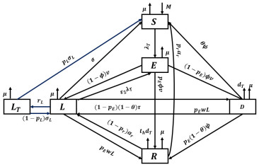
In this paper, we proposed a mathematical model for the study of tuberculosis treatment with latent treatment, taking into account the 3HP and 1HP. The model is constructed using a fractional order derivative in the Caputo sense to take advantage of the memory effect. The aim is to compare the impact on tuberculosis, whether we keep the therapies that are applied to latent tuberculosis, use of once-weekly isoniazid-rifapentine for 12 weeks (3HP), or use of isoniazid and rifapentine once a day for 28 days (1HP). We presented the basic properties of the model and found the basic reproduction number. We performed computational simulations with different fractional orders to study the behavior of the model. We studied the variation of parameters associated with new latent therapies and different treatments for active tuberculosis in the basic reproduction number. We found that the implementations have a positive impact, as the basic reproduction number remains less than unity. We showed that both implementations enable positive results because they reduce active tuberculosis in the population. The 1HP results were better and showed that the duration of treatment positively influences adherence to therapy.
- fractional derivative,
- latent,
- tuberculosis,
- therapies
Citation: Erick M. D. Moya, Diego Samuel Rodrigues. A mathematical model for the study of latent tuberculosis under 3HP and 1HP regimens[J]. Mathematical Modelling and Control, 2024, 4(4): 400-416. doi: 10.3934/mmc.2024032

Related Papers:

Abstract

In this paper, we proposed a mathematical model for the study of tuberculosis treatment with latent treatment, taking into account the 3HP and 1HP. The model is constructed using a fractional order derivative in the Caputo sense to take advantage of the memory effect. The aim is to compare the impact on tuberculosis, whether we keep the therapies that are applied to latent tuberculosis, use of once-weekly isoniazid-rifapentine for 12 weeks (3HP), or use of isoniazid and rifapentine once a day for 28 days (1HP). We presented the basic properties of the model and found the basic reproduction number. We performed computational simulations with different fractional orders to study the behavior of the model. We studied the variation of parameters associated with new latent therapies and different treatments for active tuberculosis in the basic reproduction number. We found that the implementations have a positive impact, as the basic reproduction number remains less than unity. We showed that both implementations enable positive results because they reduce active tuberculosis in the population. The 1HP results were better and showed that the duration of treatment positively influences adherence to therapy.

References

[1]	World Health Organization, Global tuberculosis report 2021, 2022. Available from: https://www.who.int/teams/global-tuberculosis-programme/tb-reports/global-tuberculosis-report-2021.
[2]	S. Swindells, R. Ramchandani, A. Gupta, C. A. Benson, J. Leon-Cruz, N. Mwelase, et al., One month of rifapentine plus isoniazid to prevent HIV-related tuberculosis, N. Engl. J. Med., 380 (2019), 1001–1011. https://doi.org/10.1056/NEJMoa1806808 doi: 10.1056/NEJMoa1806808
[3]	M. Yanes-Lane, E. Ortiz-Brizuela, J. R. Campbell, A. Benedetti, G. Churchyard, O. Oxlade, et al., Tuberculosis preventive therapy for people living with HIV: a systematic review and network meta-analysis, PLOS Med., 18 (2021), e1003738. https://doi.org/10.1371/journal.pmed.1003738 doi: 10.1371/journal.pmed.1003738
[4]	A. Malik, S. Farooq, M. Jaswal, H. Khan, K. Nasir, U. Fareed, et al., Safety and feasibility of 1 month of daily rifapentine plus isoniazid to prevent tuberculosis in children and adolescents: a prospective cohort study, Lancet, 5 (2021), 350–356. https://doi.org/10.1016/S2352-4642(21)00052-3 doi: 10.1016/S2352-4642(21)00052-3
[5]	E. M. D. Moya, A. Pietrus, S. M. Oliva, A mathematical model for the study of effectiveness in therapy in tuberculosis taking into account associated diseases, Contemp. Math., 2 (2021), 77–102. https://doi.org/10.37256/cm.212021694 doi: 10.37256/cm.212021694
[6]	E. M. D. Moya, A. Pietrus, S. M. Oliva, Mathematical model with fractional order derivatives for tuberculosis taking into account its relationship with HIV/AIDS and diabetes, Jambura J. Biomath., 2 (2021), 80–95. https://doi.org/10.34312/jjbm.v2i2.11553 doi: 10.34312/jjbm.v2i2.11553
[7]	C. K. Chong, C. Leung, W. Yew, B. C. Y. Zee, G. C. H. Tam, M. H. Wang, et al., Mathematical modelling of the impact of treating latent tuberculosis infection in the elderly in a city with intermediate tuberculosis burden, Nature, 9 (2019), 4869. https://doi.org/10.1038/s41598-019-41256-4 doi: 10.1038/s41598-019-41256-4
[8]	F. Sulayman, F. A. Abdullah, M. H. Mohd, An SVEIRE model of tuberculosis to assess the effect of an imperfect vaccine and other exogenous factors, Mathematics, 9 (2021), 327. https://doi.org/10.3390/math9040327 doi: 10.3390/math9040327
[9]	J. Andrawus, F. Y. Eguda, I. G. Usman, S. I. Maiwa, I. M. Dibal, T. G. Urum, et al., A mathematical model of a tuberculosis transmission dynamics incorporating first and second line treatment, J. Appl. Sci. Environ. Manage., 24 (2020), 917–922. https://doi.org/10.4314/jasem.v24i5.29 doi: 10.4314/jasem.v24i5.29
[10]	L. C. Barros, M. M. Lopes, F. S. Pedro, E. Esmi, J. P. C. Santos, D. E. Sánchez, The memory effect on fractional calculus: an application in the spread of COVID-19, Comput. Appl. Math., 40 (2021), 72. https://doi.org/10.1007/s40314-021-01456-z doi: 10.1007/s40314-021-01456-z
[11]	I. Podlubny, Fractional differential equations, Elsevier, 1999. https://doi.org/10.1016/s0076-5392(99)x8001-5
[12]	V. Lakshmikantham, J. V. Devi, Theory of fractional differential equations in a Banach space, Eur. J. Pure Appl. Math., 1 (2008), 38–45.
[13]	H. Kheiri, M. Jafari, Optimal control of a fractional-order model for the HIV/AIDS epidemic, Int. J. Biomath., 11 (2018), 1850086. https://doi.org/10.1142/S179352451850086 doi: 10.1142/S179352451850086
[14]	K. Diethelm, The analysis of fractional differential equations, Springer-Verlag, 2004. https://doi.org/10.1007/978-3-642-14574-2
[15]	M. Saeedian, M. Khalighi, N. Azimi-Tafreshi, G. R. Jafari, M. Ausloos, Memory effects on epidemic evolution: the susceptible-infected-recovered epidemic model, Phys. Rev. E, 95 (2017), 022409. https://doi.org/10.1103/PhysRevE.95.022409 doi: 10.1103/PhysRevE.95.022409
[16]	K. Diethelm, A fractional calculus based model for the simulation of an outbreak of dengue fever, Nonlinear Dyn., 71 (2021), 613–619. https://doi.org/10.1007/s11071-012-0475-2 doi: 10.1007/s11071-012-0475-2
[17]	V. M. Martinez, A. N. Barbosa, P. F. A. Mancera, S. Rodrigues, F. Camargo, A fractional calculus model for HIV dynamics: real data, parameter estimation and computational strategies, Chaos Solitons Fract., 152 (2021), 111398. https://doi.org/10.1016/j.chaos.2021.111398 doi: 10.1016/j.chaos.2021.111398
[18]	C. M. A. Pinto, A. R. M. Carvalho, A latency fractional order model for HIV dynamics, J. Comput. Appl. Math., 312 (2020), 240–256. https://doi.org/10.1016/j.cam.2016.05.019 doi: 10.1016/j.cam.2016.05.019
[19]	A. R. M. Carvalho, C. M. A. Pinto, D. Baleanu, HIV/HCV coinfection model: a fractional-order perspective for the effect of the HIV viral load, Adv. Differ. Equations, 2018 (2018), 2. https://doi.org/10.1186/s13662-017-1456-z doi: 10.1186/s13662-017-1456-z
[20]	W. Lin, Global existence theory and chaos control of fractional differential equations, J. Math. Anal. Appl., 332 (2007), 709–726. https://doi.org/10.1016/j.jmaa.2006.10.040 doi: 10.1016/j.jmaa.2006.10.040
[21]	O. Diekmann, J. A. P. Heesterbeek, M. G. Roberts, The construction of next-generation matrices for compartmental epidemic models, J. R. Soc. Interface, 7 (2010), 873–885. https://doi.org/10.1098/rsif.2009.0386 doi: 10.1098/rsif.2009.0386
[22]	P. van den Driessche, J. Watmough, Reproduction numbers and sub-threshold endemic equilibria for compartmental models of disease transmission, Math. Biosci., 180 (2003), 29–48. https://doi.org/10.1016/S0025-5564(02)00108-6 doi: 10.1016/S0025-5564(02)00108-6
[23]	D. Valério, A. M. Lopes, J. A. T. Machado, Entropy analysis of a railway network's complexity, Entropy, 18 (2016), 388. https://doi.org/10.3390/e18110388 doi: 10.3390/e18110388
[24]	Fatmawati, M. A. Khan, E. Bonyah, Z. Hammouch, E. M. Shaiful, A mathematical model of tuberculosis (TB) transmission with children and adults groups: a fractional model, AIMS Math., 5 (2020), 2813–2842. https://doi.org/10.3934/math.2020181 doi: 10.3934/math.2020181
[25]	C. M. A. Pinto, A. R. M. Carvalho, A latency fractional order model for HIV dynamics, J. Comput. Appl. Math., 312 (2017), 240–256. https://doi.org/10.1016/j.cam.2016.05.019 doi: 10.1016/j.cam.2016.05.019
[26]	C. Castillo-Chavez, Z. Feng, W. Huang, On the computation of $\Re_{0}$ and its role on global stability, 2001.
[27]	B. B. Gerstman, Epidemiology kept simple: an introduction to traditional and modern epidemiology, Wiley-Liss, 2003.
[28]	K. J. Rothman, Epidemiology: an introduction, Oxford University Press, 2012.
[29]	K. Diethelm, N. J. Ford, A. D. Freed, A predictor-corrector approach for the numerical solution of fractional differential equations, Nonlinear Dyn., 29 (2002), 3–22. https://doi.org/10.1023/A:1016592219341 doi: 10.1023/A:1016592219341
[30]	K. Diethelm, N. J. Ford, A. D. Freed, Detailed error analysis for a fractional Adams method, Numer. Algorithms, 36 (2004), 31–52. https://doi.org/10.1023/B:NUMA.0000027736.85078.be doi: 10.1023/B:NUMA.0000027736.85078.be
[31]	E. M. D. Moya, A. Pietrus, S. Bernard, S. P. Nuiro, A mathematical model with fractional order for obesity with positive and negative interactions and its impact on the diagnosis of diabetes, J. Math. Sci. Modell., 6 (2023), 133–149. https://doi.org/10.33187/jmsm.1339842 doi: 10.33187/jmsm.1339842

Reader Comments

Your name:*

Email:*
© 2024 the Author(s), licensee AIMS Press. This is an open access article distributed under the terms of the Creative Commons Attribution License (http://creativecommons.org/licenses/by/4.0)