Analysis of the impact of radiotherapy and surgical treatment regimens based on the SEER database on the survival outcomes of rectal cancer patients over 70 years

Wei Wang; Tongping Shen; Jiaming Wang; Wei Wang; Tongping Shen; Jiaming Wang

doi:10.3934/mbe.2024197

Mathematical Biosciences and Engineering

2024, Volume 21, Issue 3: 4463-4484. doi: 10.3934/mbe.2024197

Previous Article Next Article

Research article Special Issues

Analysis of the impact of radiotherapy and surgical treatment regimens based on the SEER database on the survival outcomes of rectal cancer patients over 70 years

1.
The First Affiliated Hospital, Anhui University of Chinese Medicine, Hefei, China
2.
School of Information Engineering, Anhui University of Chinese Medicine, Hefei, China
3.
Graduate School, Angeles University Foundation, Angeles, Philippines

Received: 21 December 2023 Revised: 05 February 2024 Accepted: 09 February 2024 Published: 27 February 2024

Objective

This study evaluates the impact of different combinations of treatment regimens, such as additional radiation, chemotherapy, and surgical treatments, on the survival of elderly rectal cancer patients ≥ 70 years of age to support physicians' clinical decision-making.

Methods

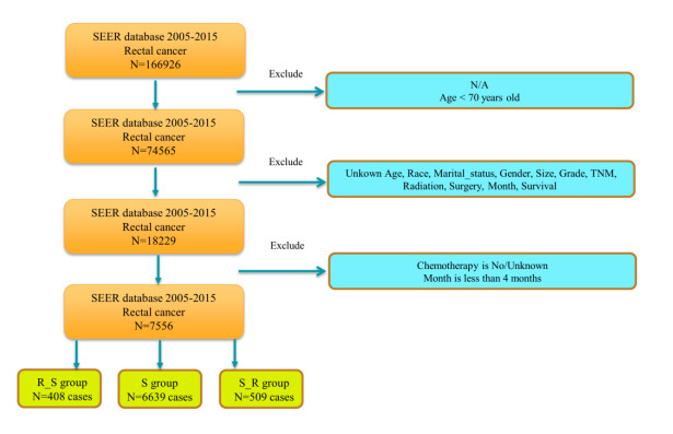
Data from a sample of elderly rectal cancer patients aged ≥ 70 years diagnosed from 2005–2015 from the US surveillance, epidemiology, and end results (SEER) database were retrospectively analyzed. The best cut-off point was selected using the x-tile software for the three continuity indices: age, tumor size, and number of regional lymph nodes. All patients were categorized into either the neoadjuvant radiotherapy and surgery group (R_S group), the surgical treatment group (S group), or the surgery and adjuvant radiotherapy group (S_R group). The propensity score allocation was used to match each included study subject in a 1:1 ratio, and the restricted mean survival time method (RMST) was used to predict the mean survival of rectal cancer patients within 5 and 10 years. The prognostic risk factors for rectal cancer patients were determined using univariate and multivariate Cox regression analyses, and nomograms were constructed. A subgroup stratification analysis of patients with different treatment combination regimens was performed using the Kaplan-Meier method, and log-rank tests were used for between-group comparisons. The model's predictive accuracy was assessed by receiver operating characteristic (ROC) curves, correction curves, and a clinical decision curve analysis (DCA).

Results

A total of 7556 cases of sample data from 2005 to 2015 were included, which were categorized into 6639 patients (87.86%) in the S group, 408 patients (5.4%) in the R_S group, and 509 patients (6.74%) in the S_R group, according to the relevant order of radiotherapy and surgery. After propensity score matching (PSM), the primary clinical characteristics of the groups were balanced and comparable. The difference in the mean survival time before and after PSM was not statistically significant in both R_S and S groups (P value > 0.05), and the difference in the mean survival time after PSM was statistically substantial in S_R and S groups (P value < 0.05). In the multifactorial Cox analysis, the M1 stage and Nodes ≥ 9 were independent risk factors. An age between 70–75 was an independent protective factor for patients with rectal cancer in the R_S and S groups. The Marital_status, T4 stage, N2 stage, M1 stage, and Nodes ≥ 9 were independent risk factors for patients with rectal cancer in the S_R and S groups, and an age between 70–81 was an independent protective factor. The ROC curve area, the model C index, and the survival calibration curve suggested good agreement between the actual and predicted values of the model. The DCA for 3-year, 5-year, and 10-year survival periods indicated that the model had some potential for application.

Conclusions

The results of the study showed no significant difference in the overall survival (OS) between elderly patients who received neoadjuvant radiotherapy and surgery and those who received surgery alone; elderly patients who received surgery and adjuvant radiotherapy had some survival benefits compared with those who received surgery alone, though the benefit of adjuvant radiotherapy was not significant. Therefore, radiotherapy for rectal cancer patients older than 70 years old should be based on individual differences in condition, and a precise treatment plan should be developed.

Keywords:

Citation: Wei Wang, Tongping Shen, Jiaming Wang. Analysis of the impact of radiotherapy and surgical treatment regimens based on the SEER database on the survival outcomes of rectal cancer patients over 70 years[J]. Mathematical Biosciences and Engineering, 2024, 21(3): 4463-4484. doi: 10.3934/mbe.2024197

Related Papers:

[1]	Walid Emam, Khalaf S. Sultan . Bayesian and maximum likelihood estimations of the Dagum parameters under combined-unified hybrid censoring. Mathematical Biosciences and Engineering, 2021, 18(3): 2930-2951. doi: 10.3934/mbe.2021148
[2]	Manal M. Yousef, Rehab Alsultan, Said G. Nassr . Parametric inference on partially accelerated life testing for the inverted Kumaraswamy distribution based on Type-II progressive censoring data. Mathematical Biosciences and Engineering, 2023, 20(2): 1674-1694. doi: 10.3934/mbe.2023076
[3]	Said G. Nassr, Amal S. Hassan, Rehab Alsultan, Ahmed R. El-Saeed . Acceptance sampling plans for the three-parameter inverted Topp–Leone model. Mathematical Biosciences and Engineering, 2022, 19(12): 13628-13659. doi: 10.3934/mbe.2022636
[4]	Wael S. Abu El Azm, Ramy Aldallal, Hassan M. Aljohani, Said G. Nassr . Estimations of competing lifetime data from inverse Weibull distribution under adaptive progressively hybrid censored. Mathematical Biosciences and Engineering, 2022, 19(6): 6252-6275. doi: 10.3934/mbe.2022292
[5]	M. G. M. Ghazal, H. M. M. Radwan . A reduced distribution of the modified Weibull distribution and its applications to medical and engineering data. Mathematical Biosciences and Engineering, 2022, 19(12): 13193-13213. doi: 10.3934/mbe.2022617
[6]	M. Nagy, M. H. Abu-Moussa, Adel Fahad Alrasheedi, A. Rabie . Expected Bayesian estimation for exponential model based on simple step stress with Type-I hybrid censored data. Mathematical Biosciences and Engineering, 2022, 19(10): 9773-9791. doi: 10.3934/mbe.2022455
[7]	Lernik Asserian, Susan E. Luczak, I. G. Rosen . Computation of nonparametric, mixed effects, maximum likelihood, biosensor data based-estimators for the distributions of random parameters in an abstract parabolic model for the transdermal transport of alcohol. Mathematical Biosciences and Engineering, 2023, 20(11): 20345-20377. doi: 10.3934/mbe.2023900
[8]	M. Nagy, Adel Fahad Alrasheedi . The lifetime analysis of the Weibull model based on Generalized Type-I progressive hybrid censoring schemes. Mathematical Biosciences and Engineering, 2022, 19(3): 2330-2354. doi: 10.3934/mbe.2022108
[9]	Ibrahim Alkhairy . Classical and Bayesian inference for the discrete Poisson Ramos-Louzada distribution with application to COVID-19 data. Mathematical Biosciences and Engineering, 2023, 20(8): 14061-14080. doi: 10.3934/mbe.2023628
[10]	Amal S. Hassan, Najwan Alsadat, Christophe Chesneau, Ahmed W. Shawki . A novel weighted family of probability distributions with applications to world natural gas, oil, and gold reserves. Mathematical Biosciences and Engineering, 2023, 20(11): 19871-19911. doi: 10.3934/mbe.2023880

Abstract

Objective

Methods

Results

Conclusions

1. Introduction

Recently, the promising attention of statisticians towards the construction of new generalized distributions has been increased to explore and develop more flexible models from the baseline models. These generalized distributions open new horizons to study real-world problems and to provide more flexibility to model the asymmetric and complex random phenomena. Therefore, several models have been developed in the literature. One of the most handy and simplest lifetime distributions induced in the statistical literature is the exponential (Ex) distribution. It has been extensively adopted for analyzing lifetime data due to its simplicity and its lack of memory property.

On the other hand, the Ex distribution with only a constant hazard rate (HR) shape is not suitable for fitting data with different HR shapes as decreasing, unimodal (upside down bathtub), increasing or bathtub shaped hazard rates which are common in reliability and engineering, among other areas. This limitation has motivated the researchers to develop more flexible extensions of the Ex model.

For more details about other methods, the interested reader can see ^{[1,2,3,4,5,6,7,8,9,10,11,12,13,14,15]}.

In the present article, we are motivated to develop a new flexible version of the Ex model called the weighted-exponential (WDEx) distribution, which can provide greater flexibility in fitting insurance data. Additionally, the aim of the article is three-fold: the first is devoted to studying a new form of the Ex distribution based on the weighted-G (WD-G) family ^[16], called the WDEx distribution. Basic distributional properties of the WDEx model are explored. The WDEx model has some desirable characteristics. It can accommodate upside-down bathtub, decreasing, decreasing-constant, increasing, and increasing-constant HR shapes. Its probability density function (PDF) possesses unimodal, right-skewed, reversed-J shape, left-skewed. The tail of the WDEx distribution is heavier than the EEx and Ex distributions as shown in Section 4 based on computational values of risk measures. The WDEx distribution can be used to model insurance data. It provides an adequate fit than other fourteen competing Ex distributions as illustrated in Section 7 for this insurance data set.

The second objective of this paper is devoted to exploring five important actuarial or risk measures, called the value at risk (VaR), tail value at risk (TVaR), tail-variance (TV), tail-variance premium (TVP), and expected shortfall (ES), for the WDEx distribution. These measures play an important role in portfolio optimization under uncertainty.

The third objective is to study the estimation of the WDEx parameters by classical and Bayesian methods. Hence, nine estimation approaches are adopted for this purpose. We explore and rank the performance of these estimators based on empirical simulation results to develop a guideline for choosing the best estimation approach for estimating the WDEx parameters.

The paper is organized in eight Sections. In Section 2, we define the WDEx model. Its basic properties are explored in Section 3. Five actuarial indicators are studies in Section 4. The model parameters are estimated using classical and Bayesian estimation in Section 5. Simulation results are provided in Section 6. Section 7 is devoted to analyzing a real-life data. Finally, some remarks are given to conclude the paper in Section 8.

2. The WDEx distribution

In this section, we define the two-parameter WDEx distribution based on the WD-G family of ^[16]. The cumulative distribution function (CDF) and PDF of the WDEx distribution has the forms

$\begin{equation} F(x) = \frac{\log \left[\left(1-e^{- \lambda x}~~\right)^{\alpha }+1\right]}{\log (2)} \end{equation}$

(2.1)

and

$\begin{equation} f(x) = \frac{\alpha \lambda e^{- \lambda x} \left(1-e^{- \lambda x}~~\right)^{\alpha -1}}{\log (2) \left[\left(1-e^{- \lambda x}~~\right)^{\alpha }+1\right]}. \end{equation}$

(2.2)

The survival function (SF), HR function (HRF) and the reversed-HRF (RHRF) are, respectively, given by

$\begin{equation} S(x) = 1-\frac{\log \left[\left(1-e^{- \lambda x}~~\right)^{\alpha }+1\right]}{\log (2)}, \end{equation}$

(2.3)

$\begin{equation} h(x) = \frac{\alpha \lambda \left(1-e^{- \lambda x}~~\right)^{\alpha }}{\left(e^{\lambda x}-1\right) \left[\left(1-e^{- \lambda x}~~\right)^{\alpha }+1\right] \left\{\log (2)-\log \left[\left(1-e^{- \lambda x}~~\right)^{\alpha }+1\right]\right\}} \end{equation}$

(2.4)

and

$\begin{equation} r(x) = \frac{\alpha \lambda e^{- \lambda x} \left(1-e^{- \lambda x}~~\right)^{\alpha -1}}{\left(\left(1-e^{- \lambda x}~~\right)^{\alpha }+1\right) \log \left(\left(1-e^{- \lambda x}~~\right)^{\alpha }+1\right)}. \end{equation}$

(2.5)

The limiting behaviors of the PDF (2.2) and HRF (2.4) are given by

$\begin{equation*} \lim\limits_{x\to0}f(x) = \begin{cases} \infty, \alpha < 1\\ 0, \; \; \alpha \geq1 \end{cases} , \lim\limits_{x\to\infty}f(x) = 0. \end{equation*}$

and

$\begin{equation*} \lim\limits_{x\to0}h(x) = \begin{cases} \infty, \alpha < 1\\ 0, \; \; \alpha \geq1 \end{cases} , \lim\limits_{x\to\infty}h(x) = \lambda. \end{equation*}$

Plots of the PDF and HRF of the WDEx distribution are illustrated in Figures 1 and 2, respectively. These graphs show that the WDEx model possesses decreasing-constant, upside-down bathtub, increasing, decreasing, and increasing-constant HR functions along with sudden spikes at the end of upside-down bathtub shape, which manages the model to analyze a non-stationary real-life data.

Figure 1. Plots of the PDF of the WDEx distribution with various parametic values.

DownLoad: Full-Size Img PowerPoint

Figure 2. Plots of the HRF of the WDEx distribution with various parametric values.

DownLoad: Full-Size Img PowerPoint

The quantile function (QF) of the WDEx distribution is given by

$\begin{equation} Q(u) = -\frac{\log \left[1-\left(2^u-1\right)^{1/\alpha }\right]}{\lambda }, \end{equation}$

(2.6)

we can determine first, second and third quartile of the WDEx distribution by setting $u = 0.25, 0.5, 0.75$ , respectively. Also, by using Eq (2.6), we can determine Bowley's skewness and Moor's kurtosis for the WDEx distribution. The WDEx skewness and kurtosis graphs for the different parametric values of $\alpha$ and $\lambda$ are shown in Figure 3.

Figure 3. Plots of the skewness and kurtosis of the WDEx model.

DownLoad: Full-Size Img PowerPoint

3. Probabilistic and statistical properties

In this section, we provide some mathematical properties of the WDEx distribution.

3.1. Linear representation

A useful linear representations of the CDF and PDF of the WDEx model are introduced in this subsection. For $-1 < x\leq1$ , we have

$\begin{equation} \log(1+x) = \sum\limits_{k = 1}^{\infty}(-1)^{k+1}\frac{x^k}{k}. \end{equation}$

(3.1)

By applying the power series (3.1) to (2.1), the CDF and PDF of the WDEx distribution can be expressed as

$\begin{align*} \label{CDF G family linear} F(x;\alpha, \lambda)& = \sum\limits_{k = 1}^{\infty} \Phi_k G_k(x)\\ \end{align*}$

and

$\begin{align*} f(x;\alpha, \lambda)& = \sum\limits_{k = 1}^{\infty} \Phi_k g_k(x), \end{align*}$

where $\Phi_k = \frac{(-1)^{k+1}}{k \log(2)}$ , $G_k(x) = \left(1-e^{- \lambda x}\right)^{\alpha k}$ and $g_k(x) = \alpha k \lambda e^{- \lambda x} \left(1-e^{- \lambda x}\right)^{\alpha k -1}$ are the CDF and PDF of the exponentiated-exponential (EEx) distribution with parameters $\lambda$ and $\alpha k$ .

3.2. Moments and generating function

The $r\text{th}$ moments of the WDEx distribution takes the form

$\begin{eqnarray*} \mu^\prime_r = E(X^r)& = &\int_{0}^{\infty} x^r f(x)dx = \sum\limits_{k = 1}^{\infty} \sum\limits_{i = 0}^{\infty} \Phi_k \frac{\alpha k \Gamma(r+1)}{\lambda^r} (-1)^i \frac{D(\alpha k-1, i)}{(i+1)^{k+1}}, \end{eqnarray*}$

where $D(a-1, b) = \frac{(a-1)\ldots(a-b)}{b!}$ . Replacing $r = 1, 2, 3$ , and $4$ in the last formula, we obtain the first four moments for the WDEx distribution.

The $n\text{th}$ moment residual life of the WDEx distribution, $E(X^n|X > x)$ , has the form

$\begin{align*} E(X^n|X > x)& = \int_{x}^{\infty} y^n f(y)dy = \sum\limits_{k = 1}^{\infty} \Phi_k \frac{\alpha \lambda k}{1-\left(1-e^{- \lambda x}\right)^{\alpha k}}\int_{x}^{\infty} y^n \exp(-\lambda y) \left(1-\exp(-\lambda y)\right)^{\alpha k-1} dy\\ & = \sum\limits_{k = 1}^{\infty} \Phi_k \frac{\alpha (-1)^n}{\lambda^n \left[1-\left(1-e^{- \lambda x}\right)^{\alpha k}\right]} \int_{0}^{\exp(-\lambda x)} (\log z)^n (1-z)^{\alpha k -1} dz, \end{align*}$

where $z = \exp(-\lambda y)$ and the mean residual life function of the proposed model is $E(X|X > x)-1$ .

the moment generating function (MGF) of the WDEx distribution is

$\begin{equation*} M(t) = \int_{0}^{\infty} e^{tx} f(x)dx = \sum\limits_{k = 1}^{\infty} \Phi_k\alpha k \beta\left(1-\frac{t}{\lambda}, \alpha k\right), \end{equation*}$

where $\beta(a, b)$ is beta function. The characteristic function of the WDEx model is

$\begin{equation*} \phi(t) = \int_{0}^{\infty} e^{itx} f(x)dx = \sum\limits_{k = 1}^{\infty} \Phi_k \alpha k \beta\left(1-\frac{it}{\lambda}, \alpha k\right). \end{equation*}$

3.3. Mean deviation, bonferroni and Lorenz curves

The mean deviation about the mean of the WDEx model reduces to

$\begin{align*} \psi_1& = \int_{0}^{\infty} |x-\mu|f(x)dx = 2\mu F(\mu)-2\mu+2\int_{\mu}^{\infty}xf(x)dx\\ & = 2\mu F(\mu)-2\mu+2\sum\limits_{k = 1}^{\infty} \Phi_k \int_{\mu}^{\infty} x g_k(x) dx = 2\mu F(\mu)-2\mu\\ &+\frac{2\alpha k}{\lambda} \sum\limits_{k = 1}^{\infty} \sum\limits_{i = 0}^{\infty} \Phi_k \frac{(-1)^i}{(i+1)^2} \binom{\alpha k -1}{i} \left[1+\mu \lambda (i+1)\right] \exp(-\mu \lambda (i+1)). \end{align*}$

The mean deviation about the median of the WDEx distribution takes the form

$\begin{align*} \psi_2& = \int_{0}^{\infty} |x-M|f(x)dx = 2\int_{M}^{\infty}xf(x) dx-\mu = 2 \sum\limits_{k = 1}^{\infty} \Phi_k \int_{M}^{\infty}x g_k(x) dx -\mu\\ & = \frac{2\alpha k}{\lambda} \sum\limits_{k = 1}^{\infty} \sum\limits_{i = 0}^{\infty} \Phi_k \frac{(-1)^i}{(i+1)^2} \binom{\alpha k -1}{i} \left[1+M \lambda (i+1)\right] \exp(-M \lambda (i+1))-\mu. \end{align*}$

The Bonferroni and Lorenz curves for a positive random variable $X$ are defined the following formulae

$\begin{align*} B(F(x))& = \frac{E(X|X\leq x)}{\mu}\\ \text{and} L(F(x))& = \frac{E(X|X\leq x) F(x)}{\mu}, \end{align*}$

where the quantity $E(X|X\leq x)$ has the form

$\begin{align*} E(X|X\leq x) = \frac{\alpha k}{\lambda F(x)} \sum\limits_{k = 1}^{\infty} \sum\limits_{i = 0}^{\infty} \Phi_k \frac{(-1)^i}{(i+1)^2} \binom{\alpha k -1}{i} \left\{1-\left[1+ \lambda (i+1)x\right] \exp(- \lambda (i+1)x)\right\}. \end{align*}$

Hence,

$\begin{align*} B(p)& = \frac{\alpha k}{\lambda p \mu} \sum\limits_{k = 1}^{\infty} \sum\limits_{i = 0}^{\infty} \Phi_k \frac{(-1)^i}{(i+1)^2} \binom{\alpha k -1}{i} \left\{1-\left[1+ \lambda (i+1)x_p\right] \exp(- \lambda (i+1)x_p)\right\} \end{align*}$

and

$\begin{align*} L(p)& = \frac{\alpha k}{\lambda \mu} \sum\limits_{k = 1}^{\infty} \sum\limits_{i = 0}^{\infty} \Phi_k \frac{(-1)^i}{(i+1)^2} \binom{\alpha k -1}{i} \left\{1-\left[1+ \lambda (i+1)x_p\right] \exp(- \lambda (i+1)x_p)\right\}, \end{align*}$

where $x_p = -\frac{\log \left[1-\left(2^p-1\right)^{1/\alpha }\right]}{\lambda }$ is the QF of the WDEx model.

3.4. Order statistics

The PDF and CDF of the $i\text{th}$ order statistic for the WDEx distribution are given by

$\begin{eqnarray*} f_{i:n}(x) & = &\frac{f(x)}{B(i, n-i+1)} \sum\limits_{h = 0}^{\infty}(-1)^h \binom{n-i}{h}F^{h+i-1}(x)\\ & = &\frac{\alpha \lambda n! \log ^{-i}(2) \left(1-e^{\lambda (-x)}\right)^{\alpha } \log ^{i-1}\left(\left(1-e^{\lambda (-x)}\right)^{\alpha }+1\right) \left(1-\frac{\log \left(\left(1-e^{\lambda (-x)}\right)^{\alpha }+1\right)}{\log (2)}\right)^{n-i}}{\Gamma (i) \left(e^{\lambda x}-1\right) \Gamma (-i+n+1) \left(\left(1-e^{\lambda (-x)}\right)^{\alpha }+1\right)} \end{eqnarray*}$

and

$\begin{eqnarray*} F_{i:n}(x) & = &\sum\limits_{r = i}^{n} (^n_r) (F(x))^r (1-F(x))^{n-r}\\ & = &\log ^{-i}(2) \binom{n}{i} \log ^i\left(\left(1-e^{\lambda (-x)}\right)^{\alpha }+1\right) \left(1-\frac{\log \left(\left(1-e^{\lambda (-x)}\right)^{\alpha }+1\right)}{\log (2)}\right)^{n-i}\\ &\times& \, _2F_1\left(1, i-n;i+1;-\frac{\log \left(\left(1-e^{-x \lambda }\right)^{\alpha }+1\right)}{\log \left(\frac{2}{\left(1-e^{-x \lambda }\right)^{\alpha }+1}\right)}\right), \end{eqnarray*}$

where $\, _2F_1\left(1, i-n; i+1;-\frac{\log \left(\left(1-e^{-x \lambda }\right)^{\alpha }+1\right)}{\log \left(\frac{2}{\left(1-e^{-x \lambda }\right)^{\alpha }+1}\right)}\right)$ is a hyper geometric function.

4. Actuarial measures

Five risk measures are explored for the WDEx distribution in this section. Some actuarial measures such as VaR, TVaR, TV, TVP, and ES are calculated. A brief simulation study for these measures is provided. Finally, an application to the insurance loss data set is analyzed. For more information we refer to refs ^{[17,18,19,20,21]}.

4.1. VaR measure

The VaR is often referred to as the quantile risk measure or the concept of quantile premium, and it is defined with a certain amount of confidence, say q (typically $90$ , $95$ , or $99\%$ ). In comparison, VaR is a quantitative sum of accumulated loss distribution. Risk management are also interested in the "chance of an unfavorable outcome" and can be represented at a specific likelihood level using the VaR. The VaR of a random variable $X$ is the $q\text{th}$ quantile of its CDF, denoted by $VaR_q$ , and it is defined by $VaR_q = Q(q)$ (see Artzner ^[22]).

The VaR measure of the WDEx distribution is expressed by

$\begin{equation*} {VaR_q = }-\frac{\log \left[1-\left(2^q-1\right)^{1/\alpha }\right]}{\lambda }. \end{equation*}$

4.2. TVaR measure

The TVaR, which is now being assigned many names, including conditional tail-expectation and conditional VaR, is another significant indicator. The TVaR is used to measure the potential value of the loss provided that there has been an occurrence outside of a provided probability level. The TVaR of a random variable $X$ is represented by

$\begin{equation*} { TVaR_q = \frac{1}{(1-q)}\int_{VaR_q}^{\infty} x\, \, f(x)dx.} \end{equation*}$

The TVaR of the WDEx distribution is

$\begin{eqnarray} TVaR_q& = &\frac{\alpha}{(1-q)\; \lambda\; \log(2)}\sum\limits_{k = 1}^{\infty}\sum\limits_{m = 1}^{\infty} \frac{(-1)^{k+1}\left[1-\left(-1+2^q\right)^{k+\frac{m}{\alpha}}\right]}{m\; k\; (m+\alpha\; k)}. \end{eqnarray}$

(4.1)

4.3. TV measure

Landsman ^[23] presented the TV risk that is described by the variance of the loss distribution beyond some critical value. The TV of the WDEx distribution is described as

$\begin{equation} TV_q(X) = E(X^2|X > x_q)-(TVaR_q)^2{ = \frac{1}{(1-q)}\int_{VaR_q}^{\infty}x^2f(x)dx-(TVaR_q)^2}, \end{equation}$

(4.2)

where

$\begin{eqnarray} E(X^2|X > x_q)& = &\frac{2\alpha}{(1-q)\; \lambda^2\; \log(2)}\sum\limits_{k = 1}^{\infty}\sum\limits_{m = 1}^{\infty}\sum\limits_{n = 1}^{k} \frac{(-1)^{k+1}\left[1-\left(-1+2^q\right)^{k+\frac{m+1}{\alpha}}\right]}{k\; n\; (m+1)\; (m+\alpha\; k+1)}, \end{eqnarray}$

(4.3)

by using Eqs (4.1)–(4.3), we get the TV of the WDEx distribution.

4.4. TVP measure

The TVP is also another effective criterion in the insurance fields. The TVP of the WDEx distribution has the form

$\begin{equation} TVP_q(x) = TVaR_q + q\; TV_q, \end{equation}$

(4.4)

where $0 < q < 1$ . The TVP of the WDEx distribution follows by replacing Eqs (4.1) and (4.2) in (4.4).

4.5. ES measure

Artzner ^[22] developed the expected shortfall (ES) as a common indicator in financial risk. In some definitions, if the underlying distribution of $X$ is continuous then the ES coincides with the Conditional tail expectation and the TVaR. The ES of the WDEx distribution takes the form

$\begin{equation} ES_q(x) = \frac{1}{q}\int_{0}^{q} VaR_t\; dt = \sum\limits_{m = 1}^{\infty}\frac{1}{q\; m\; \lambda}\int_{0}^{q}(2^t-1)^{\frac{m}{\alpha}}dt. \end{equation}$

(4.5)

4.6. Numerical simulations for risk measures

In this sub-section, we discuss some empirical results for the five aforemention risk measures for the WDEx, EEx, and Ex distributions for some parametric values. The findings are obtained through to the followings steps:

(1) Random sample of size $n = 100$ is produced from the WDEx, EEx, and Ex distributions, and their parameters are calculated via the maximum likelihood (ML) approach.

(2) 1000 Replications are designed to determine the mean of the VaR, TVaR, TV, TVP as well as ES for the three distributions.

Simulation results of the average VaR, TVaR, TV, TVP and ES for the WDEx, EEx, and Ex distributions are provided in Tables 1 and 2 and displayed graphically in Figures 4 and 5.

Table 1. Simulation results of the five measures of risk for the WDEx, EEx, and Ex distributions.

Distribution	parameter	Significance level	VaR	TVaR	TV	TVP	ES
WDEx	$\alpha=3, \, \lambda=0.5$	0.60	3.24353	5.32312	4.07298	7.83746	1.89911
		0.65	3.53435	5.59982	4.08566	8.30964	2.01350
		0.70	3.86421	5.91721	4.09951	8.82180	2.13364
		0.75	4.24850	6.29046	4.11464	9.38883	2.26146
		0.80	4.71278	6.74496	4.13115	10.03667	2.39965
		0.85	5.30475	7.32825	4.14941	10.81284	2.55232
		0.90	6.13120	8.14701	4.16895	11.82411	2.72668
		0.95	7.53258	9.54158	4.19058	13.41092	2.93856
EEx	$\alpha=3, \, \lambda=0.5$	0.60	0.49017	2.04260	3.25950	3.99830	0.11832
		0.65	0.64444	2.25379	3.35743	4.43611	0.15262
		0.70	0.84081	2.50632	3.45651	4.92587	0.19448
		0.75	1.09436	2.81518	3.55661	5.48264	0.24565
		0.80	1.43025	3.20549	3.65760	6.13157	0.30867
		0.85	1.89560	3.72427	3.75935	6.91972	0.38752
		0.90	2.59602	4.47711	3.86176	7.95269	0.48924
		0.95	3.86842	5.80090	3.96470	9.56736	0.62946
Ex	$\lambda=0.5$	0.60	1.83505	3.83774	4.05243	6.26920	0.77933
		0.65	2.10247	4.10516	4.05243	6.73924	0.87059
		0.70	2.41119	4.41388	4.05243	7.25058	0.96933
		0.75	2.77632	4.77901	4.05243	7.81833	1.07725
		0.80	3.22321	5.22590	4.05243	8.46784	1.19689
		0.85	3.79935	5.80204	4.05243	9.24660	1.33222
		0.90	4.61137	6.61406	4.05243	10.26125	1.49032
		0.95	5.99953	8.00222	4.05243	11.85203	1.68693

| Show Table

DownLoad: CSV

Table 2. Simulation results of the five measures of risk for the WDEx, EEx, and Ex distributions.

Distribution	Parameter	Significance level	VaR	TVaR	TV	TVP	ES
WDEx	$\alpha=2, \, \lambda=0.75$	0.60	1.68889	3.03197	1.78964	4.11200	0.89027
		0.65	1.87191	3.21103	1.78988	4.37915	0.95860
		0.70	2.08127	3.41720	1.79047	4.67351	1.03113
		0.75	2.32712	3.66052	1.79145	5.00516	1.10910
		0.80	2.62636	3.95782	1.79286	5.39098	1.19423
		0.85	3.01058	4.34064	1.79474	5.86253	1.28924
		0.90	3.55059	4.87971	1.79711	6.49060	1.39887
		0.95	4.47215	5.80076	1.80005	7.50092	1.53359
EEx	$\alpha=2, \, \lambda=0.75$	0.60	0.59547	1.76160	1.59250	2.71710	0.18354
		0.65	0.73107	1.91880	1.61759	2.97024	0.22029
		0.70	0.89504	2.10354	1.64237	3.25320	0.26243
		0.75	1.09725	2.32577	1.66681	3.57588	0.31110
		0.80	1.35434	2.60215	1.69096	3.95491	0.36792
		0.85	1.69752	2.96394	1.71477	4.42150	0.43550
		0.90	2.19695	3.48134	1.73829	5.04581	0.51848
		0.95	3.07660	4.37836	1.76151	6.05179	0.62721
Ex	$\lambda=0.75$	0.60	1.13884	2.38172	1.56099	3.31832	0.48365
		0.65	1.30481	2.54769	1.56099	3.56233	0.54029
		0.70	1.49640	2.73928	1.56100	3.83198	0.60157
		0.75	1.72300	2.96588	1.56099	4.13662	0.66855
		0.80	2.00034	3.24322	1.56099	4.49202	0.74280
		0.85	2.35790	3.60078	1.56099	4.92762	0.82678
		0.90	2.86184	4.10472	1.56099	5.50962	0.92490
		0.95	3.72334	4.96623	1.56099	6.44917	1.04692

| Show Table

DownLoad: CSV

Figure 4. The above figure displays the graphs of the VaR, TVaR, TV, TVP, and ES using the values in Table 1.

DownLoad: Full-Size Img PowerPoint

Figure 5. The above figure displays the graphs of the VaR, TVaR, TV, TVP, and ES using the values in Table 2.

DownLoad: Full-Size Img PowerPoint

The model with highest value of VaR, TVaR, TV, TVP and ES metrics does also have a heavier tail than other competitor models. The results illustrate that the WDEx model has improved quantities of the five risk factors than the EEx, and Ex distributions. Thus, the WDEx model with these parameter values has a heavier-tail than other distributions and could be used efficiently to model heavy-tailed insurance data.

5. Classical and Bayesian estimation

This section is devoted to address the estimation of the WDEx parameters by various estimation methods including eight classical estimation approaches, such as the MLE, Anderson–Darling (ADE) and right-tail Anderson–Darling (RTADE), Cramér–von Mises (CVME), least-squares (LSE), weighted least-squares (WLSE), maximum product of spacings (MPS) and percentile estimation (PCE), and Bayesian approach under three loss functions namely, square error (SE), linear exponential (LINEX), and the general entropy (GE).

Consider the random sample of size $n$ , say $x_1, x_2, \ldots, x_n$ , from the PDF (2.2), and let $x_{1:n}, x_{2:n}, \ldots, x_{2:n}$ be their associated order statistics.

5.1. Maximum likelihood

The log-likelihood function of the WDEx distribution has the form

$\begin{equation} L = (\alpha -1) \sum\limits _{i = 1}^n \log \left((1-e)^{-\lambda x_i}\right)-\sum\limits _{i = 1}^n \log \left(\left(1-e^{-\lambda x_i}\right){}^{\alpha }+1\right)-\lambda \sum\limits _{i = 1}^n x_i+n \log \left(\frac{\alpha \lambda }{\log (2)}\right). \end{equation}$

(5.1)

Hence, the MLEs of $\alpha$ and $\lambda$ are determined by maximizing Eq (5.1) with respect to $\alpha$ and $\lambda$ , as the solutions of the following equations

$\begin{equation*} \frac{\partial L}{\partial \alpha} = -\sum \limits_{i = 1}^n \frac{\left(1-e^{-\lambda x_i}\right){}^{\alpha } \log \left(1-e^{-\lambda x_i}\right)}{\left(1-e^{-\lambda x_i}\right){}^{\alpha }+1}+\sum \limits_{i = 1}^n \log \left((1-e)^{-\lambda x_i}\right)+\frac{n}{\alpha } = 0 \end{equation*}$

and

$\begin{align*} \frac{\partial L}{\partial \lambda}& = (\alpha -1) \sum _{i = 1}^n \frac{x_i e^{-\lambda x_i}}{1-e^{-\lambda x_i}}-\sum _{i = 1}^n \frac{\alpha x_i e^{-\lambda x_i} \left(1-e^{-\lambda x_i}\right){}^{\alpha -1}}{\left(1-e^{-\lambda x_i}\right){}^{\alpha }+1}-\sum _{i = 1}^n x_i+\frac{n}{\lambda } = 0. \end{align*}$

Furthermore, solving the above two equations mathematically is complicated, hence the equations can be solved by the numerical methods to obtain the MLE of $\alpha$ and $\lambda$ .

5.2. Ordinary and weighted least-squares

The LSE of the WDEx parameters come from minimizing

$\begin{equation*} O = \sum\limits_{i = 1}^{n}\left[F(x_{i:n})-\frac{i}{n+1}\right]^2 = \sum\limits_{i = 1}^{n}\left[\frac{\log \left[\left(1-e^{- \lambda x_{i:n}}\right)^{\alpha }+1\right]}{\log (2)}-\frac{i}{n+1}\right]^2. \end{equation*}$

The LSE of the WDEx parameters are also obtained by solving the following equations

$\begin{equation*} \sum\limits_{i = 1}^{n}\left\{\frac{\log \left[\left(1-e^{- \lambda x_{i:n}}\right)^{\alpha }+1\right]}{\log (2)}-\frac{i}{n+1}\right\}\varDelta_s (x_{i:n}) = 0, \quad s = 1, 2, \end{equation*}$

where

$\begin{eqnarray} \varDelta_1 (x_{i:n})& = & \frac{\partial}{\partial \alpha}F(x_{i:n}) = \frac{\left(1-e^{-\lambda x_i}\right){}^{\alpha } \log \left(1-e^{-\lambda x_i}\right)}{\log (2) \left(\left(1-e^{-\lambda x_i}\right){}^{\alpha }+1\right)}, \end{eqnarray}$

(5.2)

$\begin{eqnarray} \varDelta_2 (x_{i:n})& = &\frac{\partial}{\partial \lambda}F(x_{i:n}) = \frac{\alpha x_i e^{-\lambda x_i} \left(1-e^{-\lambda x_i}\right){}^{\alpha -1}}{\log (2) \left(\left(1-e^{-\lambda x_i}\right){}^{\alpha }+1\right)}. \end{eqnarray}$

(5.3)

The WLSE of the WDEx parameters can be calculated by minimizing

$\begin{equation*} W = \sum\limits_{i = 1}^{n}\frac{(n+1)^2(n+2)}{i(n-i+1)}\left[F(x_{i:n})-\frac{i}{n+1}\right]^2 = \sum\limits_{i = 1}^{n}\frac{(n+1)^2(n+2)}{i(n-i+1)}\left[\frac{\log \left[\left(1-e^{- \lambda x_{i:n}}\right)^{\alpha }+1\right]}{\log (2)}-\frac{i}{n+1}\right]^2. \end{equation*}$

Furthermore, the WLSE of the WDEx parameters are obtained by solving the following equations

$\begin{equation*} \sum\limits_{i = 1}^{n}\frac{(n+1)^2(n+2)}{i(n-i+1)}\left[\frac{\log \left[\left(1-e^{- \lambda x_{i:n}}\right)^{\alpha }+1\right]}{\log (2)}-\frac{i}{n+1}\right] \varDelta_s (x_{i:n}) = 0, \end{equation*}$

where $\varDelta_s (x_{i:n}), s = 1, 2, 3$ are given by Eqs (5.2) and (5.3).

5.3. Anderson-Darling and right-tail Anderson-Darling

The ADE of the WDEx parameters are obtained by minimizing

$\begin{equation*} A = -n-\frac{1}{n}\sum\limits_{i = 1}^{n}(2i-1)[\log F(x_{i:n})+\log S(x_{i:n})]. \end{equation*}$

The ADE are also calculated by solving the following equations

$\begin{equation*} \sum\limits_{i = 1}^{n}(2i-1)\left[\frac{\varDelta_s (x_{i:n})}{F(x_{i:n})}-\frac{\varDelta_s (x_{n+1-i:n})}{S(x_{n+1-i:n})}\right] = 0, \end{equation*}$

where $\varDelta_s (x_{i:n}), s = 1, 2, 3$ were defined in (5.2) and (5.3), respectively.

The RTADE of the WDEx parameters can be calculated by minimizing

$\begin{equation*} R = \frac{n}{2}-2\sum\limits_{i = 1}^{n}F(x_{i:n})-\frac{1}{n}\sum\limits_{i = 1}^{n}(2i-1)\log S(x_{i:n}). \end{equation*}$

The RADE can also be follow by solving the non-linear equations

$\begin{equation*} -2\sum\limits_{i = 1}^{n}\varDelta_s (x_{n+1-i:n}) +\frac{1}{ n}\sum\limits_{i = 1}^{n}\frac{\varDelta_s (x_{n+1-i:n})}{S(x_{n+1-i:n})} = 0, \end{equation*}$

where $\varDelta_s (x_{i:n}), s = 1, 2, 3$ are defined in (5.2) and (5.3).

5.4. Maximum product of spacings

As an alternative to the ML method, the maximum product spacing (MPS) approach is adopted to estimate the parameters of continuous univariate distributions. The uniform spacings, say $D_i$ , of a random sample of size $n$ from the WDEx distribution are defined by

$\begin{equation*} D_i = F(x_{i})-F(x_{i-1}), \, \, i = 1, 2, ..., n. \end{equation*}$

where $F(x_0) = 0$ , $F(x_{n+1} = 1)$ and $\sum_{i = 1}^{n+1} D_i = 1$ . Then, the MPSE of the WDEx parameters can be obtained by maximizing

$\begin{equation*} G = \frac{1}{n+1} \sum\limits_{i = 1}^{n+1} \log(D_i), \end{equation*}$

with respect to $\alpha$ and $\lambda$ . Further, the MPSE of the WDEx parameters are also obtained by solving

$\begin{equation*} \frac{1}{n+1} \sum\limits_{i = 1}^{n+1} \frac{1}{D_i} [\varDelta_s (x_{i:n})-\varDelta_s (x_{i-1:n})] = 0, \end{equation*}$

where $\varDelta_s (x_{i:n}), s = 1, 2, 3$ are presented in (5.2) and (5.3).

5.5. Percentile estimation

Let $p_i = \frac{i}{n+1}$ be an estimate of $F(x_{i:n})$ . Hence, the PCE of the WDEx parameters are obtained by minimizing

$\begin{equation*} PCE = \sum\limits_{i = 1}^{n}[x_{i:n}-Q(p_i)]^2 = \sum\limits_{i = 1}^{n}\left[x_{i:n}-\frac{\log \left[1-\left(2^{p_i}-1\right)^{1/\alpha }\right]}{\lambda }\right]^2. \end{equation*}$

The PCE are calculated by solving the following equations

$\begin{equation*} \sum\limits_{i = 1}^{n}\left(x_{i:n}-\frac{\log \left[1-\left(2^{p_i}-1\right)^{1/\alpha }\right]}{\lambda }\right)\varPhi_s(x_{i:n}) = 0, \quad s = 1, 2, \end{equation*}$

where

$\begin{eqnarray*} \varPhi_1 (x_{i:n})& = & \frac{\partial}{\partial \alpha}Q(p_i) = \frac{\left(2^{p_i}-1\right){}^{1/\alpha } \log \left(2^{p_i}-1\right)}{\alpha ^2 \lambda \left(\left(2^{p_i}-1\right){}^{1/\alpha }-1\right)}, \\ \varPhi_2 (x_{i:n})& = & \frac{\partial}{\partial \lambda}Q(p_i) = \frac{\log \left(1-\left(2^{p_i}-1\right){}^{1/\alpha }\right)}{\lambda ^2}. \end{eqnarray*}$

5.6. Cramér–von mises

The CVME of the WDEx parameters are obtained by minimizing

$\begin{equation*} CV = \frac{1}{12n}+\sum\limits_{i = 1}^{n}\left[F(x_{i:n})-\frac{2i-1}{2n}\right]^2 = \frac{1}{12n}+\sum\limits_{i = 1}^{n}\left[\frac{\log \left[\left(1-e^{- \lambda x_{i:n}}\right)^{\alpha }+1\right]}{\log (2)}-\frac{2i-1}{2n}\right]^2, \end{equation*}$

They also are obtained by solving the following equations

$\begin{equation*} \sum\limits_{i = 1}^{n}\left\{\frac{\log \left[\left(1-e^{- \lambda x_{i:n}}\right)^{\alpha }+1\right]}{\log (2)}-\frac{2i-1}{2n}\right\} \varDelta_s (x_{i:n}) = 0, \end{equation*}$

where $\varDelta_s (x_{i:n}), s = 1, 2, 3$ are given in (5.2) and (5.3).

5.7. Bayesian estimation

The Bayesian estimation (BE) for the distribution parameters under different loss functions such as the SE, LINEX, and GE loss functions is studied. The parameters are assumed to have gamma priors. Thus,

$\pi_{1}(\alpha) \propto \alpha^{\mu_{1}-1}e^{\frac{-\alpha}{\lambda_{1}}}, \;\;\;\; \alpha > 0, \;\mu_{1}, \lambda_{1} > 0$

and

$\pi_{2}(\lambda) \propto \lambda^{\mu_{2}-1}e^{\frac{-\lambda}{\lambda_{2}}}, \;\;\;\; \lambda > 0\;\mu_{2}, \lambda_{2} > 0$

Suppose that the parameters are independent, therefore the joint PDF of the prior distribution has the form

$\begin{equation} \pi(\alpha, \lambda)\propto \lambda^{\mu_{2}-1}\alpha^{\mu_{1}-1}e^{-(\frac{\alpha}{\lambda_{1}}+\frac{\lambda}{\lambda_2})}. \end{equation}$

(5.4)

The posterior density function of the parameters $\alpha$ and $\lambda$ can be obtained from (5.1) and (5.4), as follows

$\begin{equation} \begin{split} \pi^{*}(\Theta|{t}) = \pi^{*}(\alpha, \lambda|{t}) & \propto L(\alpha, \lambda )\;\pi(\alpha, \lambda).\\ \end{split} \end{equation}$

(5.5)

The BE of the function of parameters $U = U(\Theta)$ , $\Theta = (\gamma, \alpha, \theta_{1}, b)$ under the SE loss function (LF) is given by

$\begin{equation} \hat{U}_{SE} = \underset{\Theta}{\int} U \;\pi^{*}(\Theta|{t}) \;d\Theta. \end{equation}$

(5.6)

Under the LINEX LF, the BE of $U = U(\Theta)$ reduces to

$\begin{equation} \hat{U}_{LINEX} = -\frac{1}{c}\log \left[\underset{\Theta}{\int} e^{-c U} \;\pi^{*}(\Theta|{t}) \;d\Theta\right], \end{equation}$

(5.7)

where $c\neq 0$ is the shape parameter of the LINEX LF.

Based on the GE LF, the BE of $U$ takes the form

$\begin{equation} \hat{U}_{GE} = \left(\underset{\Theta}{\int} U^{-q} \pi^{*}(\Theta|{t}) d\Theta \right)^{-1/q}, \end{equation}$

(5.8)

where $q \neq 0$ .

It is obvious that the integrals in Eqs (5.6)–(5.8) are complicated. Consequently, the important sampling method and the MCMC method are applied to obtain an approximation for these integrals. The Metropolis Hasting (MH) algorithm produces a series of draws from the WDEx distribution as follows:

Algorithm 1 The MCMC for BE

1. First we will start with initial values for the two parameters

$\alpha^{(0)}=\hat{\alpha}_{MLE},$

$\lambda^{(0)}=\hat{\lambda}_{MLE},$

2. Start the first iteration with counter

$i=1.$

3. Now we will generate a random value for

$\alpha^{*}$ from proposal distribution

$\textbf{N}(\alpha^{(i-1)}, var(\alpha^{(i-1)}))$ ., where

$var(\alpha^{(i-1)})$ is the variance of the parameter

$\alpha$

4. We will use the following equation

$A(\alpha^{(i-1)}|\alpha^{*})=\min\left[1, \frac{\pi^{*}(\alpha^{*}|\lambda^{(i-1)})} {\pi^{*}(\alpha^{(i-1)}|\lambda^{(i-1)})}\right]$ , the value of this equation donates the acceptance probability.

5. Now we will generate a random value that follows the uniform distribution

$U\thicksim U(0, 1)$ that ranges from 0 to 1.

6. If

$U\leq A(\alpha^{(i-1)}|\alpha^{*}),$ put

$\alpha^{(i)}=\alpha^{*}$ , else put

$\alpha^{(i)}=\alpha^{(i-1)}$ .

7. In order to evaluate the other parameter

$\lambda$ we will repeat the steps from ((2)–(6)) for

$\lambda$ .

8. Now increase the counter by one such that

$i=i+1$ .

9. To avoid any correlation between the initial values and the estimated values we will repeat the steps from ((3)–(8)),

$N=10, 000$ times to obtain

$(\alpha^{(1)}, \lambda^{(1)})$ , ...,

$(\alpha^{(N)}, \beta^{(N)})$ .

Then, the BEs of

$u(\alpha, \beta)$ using the MCMC under the three LFs are, respectively, given by

$\tilde{u}_{SE}=\frac{1}{N-M}\sum\limits_{i=M+1}^{N}u(\alpha^{(i)}, \lambda^{(i)}),$

$\tilde{u}_{LINEX}=-\frac{1}{c}\log\left[\frac{1}{N-M}\sum\limits_{i=M+1}^{N}\exp\{-c\; u(\alpha^{(i)}, \lambda^{(i)})\}\right]$

and

$\tilde{u}_{GE}=\left[\frac{1}{N-M}\sum\limits_{i=M+1}^{N}(u(\alpha^{(i)}, \lambda^{(i)}))^{-q}\right]^{-1/q},$

where

$M=2000$ is the burn-in period.

| Show Table

DownLoad: CSV

5.8. TK-approximation for Bayesian estimates

One of the most computationally efficient methods, for estimating the distribution parameter is the Tierney and Kadane ^[24] (TK) method. They developed an easily calculable integration approximation approach for evaluating the distribution parameters. The advantage of the TK approach is that it provides an easy and fast approximation method, however some methods are very hard to find the values of integration and takes a lot of time and effort.

Throughout this segment, we use the TK approximation method for calculating the Bayesian estimates (BEs) of the parameters that are focused on the SE, Linex, and GE LFs. TK method ^[24] is among the techniques to obtain the estimated value of the ratio of the two integrals as given in the following equation

$\begin{equation} \hat{U}(\Theta) = \frac{\underset{\Theta}{\int} U(\Theta) \;e^{\left[ l(\Theta|{t})+\rho(\Theta|{t})\right]} ~~\;d\Theta}{\underset{\Theta}{\int} e^{\left[ l(\Theta|{t})+\rho(\Theta|{t})\right]}~~ \;d\Theta}, \end{equation}$

(5.9)

where $U(\Theta)$ is any function of the parameters $(\alpha, \lambda)$ , $l(\Theta|{t})$ is defined in (5.1), and $\rho(\Theta|{t})$ is the logarithm joint prior distribution which is defined by

$\begin{eqnarray} \rho(\alpha, \lambda|{t})& = &(\mu_1-1) ln(\alpha)+(\mu_2-1) ln\lambda \\ &-&\left(\frac{\alpha}{\lambda_1}+\frac{\lambda}{\lambda_2}\right). \end{eqnarray}$

(5.10)

To obtain an explicit expression for $\hat{U}_{SE}(\Theta)$ using TK approximation, we consider the following functions

$\begin{equation} \delta(\Theta) = \frac{l(\Theta|{t})+\rho(\Theta|{t})}{n} \end{equation}$

(5.11)

and

$\begin{equation} \delta^*(\Theta) = \delta(\Theta)+\frac{ln U(\Theta)}{n}. \end{equation}$

(5.12)

Now, assume that the following groups of values $(\hat{\alpha}_{\delta}, \hat{\lambda}_{\delta})$ and $(\hat{\alpha}_{\delta^*}, \hat{\lambda}_{\delta^*})$ maximize the functions $\delta(\alpha, \lambda)$ and $\delta^*(\alpha, \lambda)$ , respectively.

Hence, we can evaluate the approximation of $\hat{U}(\Theta)$ by

$\begin{equation} \hat{U}_{TK}(\Theta) = \sqrt{\frac{|\Delta^*|}{|\Delta|}} \exp{\left[n \left\{\delta(\hat{\alpha}_{\delta}, \hat{\lambda}_{\delta})-\delta(\hat{\alpha}_{\delta^*}, \hat{\lambda}_{\delta^*})\right\}\right]}, \end{equation}$

(5.13)

where $|\Delta|$ and $|\Delta^*|$ refers to the determinants of negative inverse hessian of $\delta(\alpha, \lambda)$ and $\delta^*(\alpha, \lambda)$ , respectively.

6. Simulation results

Now, we asses the performance of the above estimation techniques in estimating the WDEx parameters using simulation results. Different sample sizes, $n = \{15, 30, 70, 100, 200, 350\}$ , and some initial values are assigned. We generated $5000$ random samples from the WDEx distribution to calculate the average absolute biases (ABBs), mean square errors (MSEs), and mean relative errors of estimates (MREs) using the R program©.

The following respective mathematical formulae are used to evaluate the ABBs, MSEs, and MREs (for $\pmb \theta = (\alpha, \lambda)^{'}$ )

$\begin{equation*} ABs = \frac{1}{N}\sum\limits_{i = 1}^{N}|\widehat{\pmb \theta}-\pmb \theta|, \, \, \, \, MSEs = \frac{1}{N}\sum\limits_{i = 1}^{N}(\widehat{\pmb \theta}-\pmb \theta)^2, \, \, \, \, MREs = \frac{1}{N}\sum\limits_{i = 1}^{N}|\widehat{\pmb \theta}-\pmb \theta|/\pmb \theta. \end{equation*}$

Table 3 reports the simulation results including the ABBs, MSEs, and MREs of the WDEx parameters using the nine estimation approaches. One can note that all methods provide small ABBs, MSEs and MREs in all parametric values. The nine estimators are consistent, i.e., the MSEs decrease as the sample size increases, for all studied cases.

Table 3. Simulation results of the WDEx distribution using different estimators for (

$\alpha = 0.75, \; \lambda = 0.75$ ).

n	Est.	Est. Par.	Classical
n	Est.	Est. Par.	MLE	ADE	CVME	MPS	LSE	PCE	RTADE	WLSE
15	BIAS	$\hat{\alpha}$	$0.25192877 ^{\{ 5 \}\{ 11 \}}$	$0.22405917 ^{\{ 2 \}\{ 8 \}}$	$0.30164256 ^{\{ 7 \}\{ 13 \}}$	$0.19839734 ^{\{ 1 \}\{ 7 \}}$	$0.24557181 ^{\{ 4 \}\{ 10 \}}$	$0.32687545 ^{\{ 8 \}\{ 14 \}}$	$0.29638657 ^{\{ 6 \}\{ 12 \}}$	$0.24157906 ^{\{ 3 \}\{ 9 \}}$
		$\hat{\lambda}$	$0.32093518 ^{\{ 5 \}\{ 11 \}}$	$0.30428638 ^{\{ 2 \}\{ 8 \}}$	$0.39524432 ^{\{ 8 \}\{ 14 \}}$	$0.26371696 ^{\{ 1 \}\{ 7 \}}$	$0.31652453 ^{\{ 4 \}\{ 10 \}}$	$0.34677645 ^{\{ 7 \}\{ 13 \}}$	$0.32593945 ^{\{ 6 \}\{ 12 \}}$	$0.31219147 ^{\{ 3 \}\{ 9 \}}$
	MSE	$\hat{\alpha}$	$0.16122813 ^{\{ 3 \}\{ 9 \}}$	$0.11215242 ^{\{ 2 \}\{ 8 \}}$	$0.26608275 ^{\{ 8 \}\{ 14 \}}$	$0.06560425 ^{\{ 1 \}\{ 7 \}}$	$0.1682729 ^{\{ 4 \}\{ 10 \}}$	$0.19013447 ^{\{ 6 \}\{ 12 \}}$	$0.22921014 ^{\{ 7 \}\{ 13 \}}$	$0.18043259 ^{\{ 5 \}\{ 11 \}}$
		$\hat{\lambda}$	$0.21915477 ^{\{ 4 \}\{ 10 \}}$	$0.20639267 ^{\{ 2 \}\{ 8 \}}$	$0.34394628 ^{\{ 8 \}\{ 14 \}}$	$0.11724707 ^{\{ 1 \}\{ 7 \}}$	$0.2237624 ^{\{ 5 \}\{ 11 \}}$	$0.2148123 ^{\{ 3 \}\{ 9 \}}$	$0.23978318 ^{\{ 7 \}\{ 13 \}}$	$0.23922943 ^{\{ 6 \}\{ 12 \}}$
	MRE	$\hat{\alpha}$	$0.33590503 ^{\{ 5 \}\{ 11 \}}$	$0.29874556 ^{\{ 2 \}\{ 8 \}}$	$0.40219008 ^{\{ 7 \}\{ 13 \}}$	$0.26452979 ^{\{ 1 \}\{ 7 \}}$	$0.32742908 ^{\{ 4 \}\{ 10 \}}$	$0.43583393 ^{\{ 8 \}\{ 14 \}}$	$0.3951821 ^{\{ 6 \}\{ 12 \}}$	$0.32210541 ^{\{ 3 \}\{ 9 \}}$
		$\hat{\lambda}$	$0.42791357 ^{\{ 5 \}\{ 11 \}}$	$0.40571517 ^{\{ 2 \}\{ 8 \}}$	$0.52699243 ^{\{ 8 \}\{ 14 \}}$	$0.35162261 ^{\{ 1 \}\{ 7 \}}$	$0.42203271 ^{\{ 4 \}\{ 10 \}}$	$0.4623686 ^{\{ 7 \}\{ 13 \}}$	$0.43458594 ^{\{ 6 \}\{ 12 \}}$	$0.4162553 ^{\{ 3 \}\{ 9 \}}$
	$\sum CRanks$		$27 ^{\{ 5 \}}$	$12 ^{\{ 2 \}}$	$46 ^{\{ 8 \}}$	$6 ^{\{ 1 \}}$	$25 ^{\{ 4 \}}$	$39 ^{\{ 7 \}}$	$38 ^{\{ 6 \}}$	$23 ^{\{ 3 \}}$
	$\sum C\&BRanks$		$63 ^{\{ 11 \}}$	$48 ^{\{ 8 \}}$	$82 ^{\{ 14 \}}$	$42 ^{\{ 7 \}}$	$61 ^{\{ 10 \}}$	$75 ^{\{ 13 \}}$	$74 ^{\{ 12 \}}$	$59 ^{\{ 9 \}}$
30	BIAS	$\hat{\alpha}$	$0.14405974 ^{\{ 3 \}\{ 9 \}}$	$0.13901101 ^{\{ 2 \}\{ 8 \}}$	$0.17725422 ^{\{ 7 \}\{ 13 \}}$	$0.13213658 ^{\{ 1 \}\{ 7 \}}$	$0.16209531 ^{\{ 5 \}\{ 11 \}}$	$0.25820992 ^{\{ 8 \}\{ 14 \}}$	$0.16964029 ^{\{ 6 \}\{ 12 \}}$	$0.14580412 ^{\{ 4 \}\{ 10 \}}$
		$\hat{\lambda}$	$0.18969311 ^{\{ 2 \}\{ 8 \}}$	$0.19141061 ^{\{ 3 \}\{ 9 \}}$	$0.23350009 ^{\{ 7 \}\{ 13 \}}$	$0.18115544 ^{\{ 1 \}\{ 7 \}}$	$0.22786428 ^{\{ 6 \}\{ 12 \}}$	$0.24136118 ^{\{ 8 \}\{ 14 \}}$	$0.20026589 ^{\{ 4 \}\{ 10 \}}$	$0.20766574 ^{\{ 5 \}\{ 11 \}}$
	MSE	$\hat{\alpha}$	$0.03746839 ^{\{ 3 \}\{ 9 \}}$	$0.03635968 ^{\{ 2 \}\{ 8 \}}$	$0.06052504 ^{\{ 7 \}\{ 13 \}}$	$0.02548745 ^{\{ 1 \}\{ 7 \}}$	$0.05095711 ^{\{ 5 \}\{ 11 \}}$	$0.10729773 ^{\{ 8 \}\{ 14 \}}$	$0.05828137 ^{\{ 6 \}\{ 12 \}}$	$0.04260275 ^{\{ 4 \}\{ 10 \}}$
		$\hat{\lambda}$	$0.06746508 ^{\{ 3 \}\{ 9 \}}$	$0.06525692 ^{\{ 2 \}\{ 8 \}}$	$0.09980727 ^{\{ 8 \}\{ 14 \}}$	$0.04907736 ^{\{ 1 \}\{ 7 \}}$	$0.09345408 ^{\{ 7 \}\{ 13 \}}$	$0.09161708 ^{\{ 6 \}\{ 12 \}}$	$0.07713619 ^{\{ 4 \}\{ 10 \}}$	$0.0814058 ^{\{ 5 \}\{ 11 \}}$
	MRE	$\hat{\alpha}$	$0.19207965 ^{\{ 3 \}\{ 9 \}}$	$0.18534802 ^{\{ 2 \}\{ 8 \}}$	$0.23633896 ^{\{ 7 \}\{ 13 \}}$	$0.1761821 ^{\{ 1 \}\{ 7 \}}$	$0.21612709 ^{\{ 5 \}\{ 11 \}}$	$0.34427989 ^{\{ 8 \}\{ 14 \}}$	$0.22618705 ^{\{ 6 \}\{ 12 \}}$	$0.19440549 ^{\{ 4 \}\{ 10 \}}$
		$\hat{\lambda}$	$0.25292415 ^{\{ 2 \}\{ 8 \}}$	$0.25521415 ^{\{ 3 \}\{ 9 \}}$	$0.31133346 ^{\{ 7 \}\{ 13 \}}$	$0.24154058 ^{\{ 1 \}\{ 7 \}}$	$0.30381904 ^{\{ 6 \}\{ 12 \}}$	$0.32181491 ^{\{ 8 \}\{ 14 \}}$	$0.26702119 ^{\{ 4 \}\{ 10 \}}$	$0.27688765 ^{\{ 5 \}\{ 11 \}}$
	$\sum CRanks$		$16 ^{\{ 3 \}}$	$14 ^{\{ 2 \}}$	$43 ^{\{ 7 \}}$	$6 ^{\{ 1 \}}$	$34 ^{\{ 6 \}}$	$46 ^{\{ 8 \}}$	$30 ^{\{ 5 \}}$	$27 ^{\{ 4 \}}$
	$\sum C\&BRanks$		$52 ^{\{ 9 \}}$	$50 ^{\{ 8 \}}$	$79 ^{\{ 13 \}}$	$42 ^{\{ 7 \}}$	$70 ^{\{ 12 \}}$	$82 ^{\{ 14 \}}$	$66 ^{\{ 11 \}}$	$63 ^{\{ 10 \}}$
70	BIAS	$\hat{\alpha}$	$0.08792199 ^{\{ 3 \}\{ 9 \}}$	$0.08650543 ^{\{ 2 \}\{ 8 \}}$	$0.10310607 ^{\{ 6 \}\{ 12 \}}$	$0.08281633 ^{\{ 1 \}\{ 7 \}}$	$0.10074083 ^{\{ 5 \}\{ 11 \}}$	$0.1753952 ^{\{ 8 \}\{ 14 \}}$	$0.10421227 ^{\{ 7 \}\{ 13 \}}$	$0.08803723 ^{\{ 4 \}\{ 10 \}}$
		$\hat{\lambda}$	$0.11408442 ^{\{ 1 \}\{ 7 \}}$	$0.12445549 ^{\{ 3 \}\{ 9 \}}$	$0.14143312 ^{\{ 7 \}\{ 13 \}}$	$0.1164039 ^{\{ 2 \}\{ 8 \}}$	$0.13839689 ^{\{ 6 \}\{ 12 \}}$	$0.16478766 ^{\{ 8 \}\{ 14 \}}$	$0.12896275 ^{\{ 5 \}\{ 11 \}}$	$0.12549479 ^{\{ 4 \}\{ 10 \}}$
	MSE	$\hat{\alpha}$	$0.01336042 ^{\{ 3 \}\{ 9 \}}$	$0.01302739 ^{\{ 2 \}\{ 8 \}}$	$0.01826087 ^{\{ 6 \}\{ 12 \}}$	$0.01051127 ^{\{ 1 \}\{ 7 \}}$	$0.01740773 ^{\{ 5 \}\{ 11 \}}$	$0.04721909 ^{\{ 8 \}\{ 14 \}}$	$0.01897672 ^{\{ 7 \}\{ 13 \}}$	$0.01339529 ^{\{ 4 \}\{ 10 \}}$
		$\hat{\lambda}$	$0.02286488 ^{\{ 2 \}\{ 8 \}}$	$0.02612201 ^{\{ 3 \}\{ 9 \}}$	$0.03569504 ^{\{ 7 \}\{ 13 \}}$	$0.02027791 ^{\{ 1 \}\{ 7 \}}$	$0.03209949 ^{\{ 6 \}\{ 12 \}}$	$0.04224291 ^{\{ 8 \}\{ 14 \}}$	$0.02824455 ^{\{ 5 \}\{ 11 \}}$	$0.02671826 ^{\{ 4 \}\{ 10 \}}$
	MRE	$\hat{\alpha}$	$0.11722932 ^{\{ 3 \}\{ 9 \}}$	$0.11534057 ^{\{ 2 \}\{ 8 \}}$	$0.13747476 ^{\{ 6 \}\{ 12 \}}$	$0.11042178 ^{\{ 1 \}\{ 7 \}}$	$0.13432111 ^{\{ 5 \}\{ 11 \}}$	$0.23386027 ^{\{ 8 \}\{ 14 \}}$	$0.13894969 ^{\{ 7 \}\{ 13 \}}$	$0.11738297 ^{\{ 4 \}\{ 10 \}}$
		$\hat{\lambda}$	$0.15211257 ^{\{ 1 \}\{ 7 \}}$	$0.16594066 ^{\{ 3 \}\{ 9 \}}$	$0.18857749 ^{\{ 7 \}\{ 13 \}}$	$0.1552052 ^{\{ 2 \}\{ 8 \}}$	$0.18452919 ^{\{ 6 \}\{ 12 \}}$	$0.21971689 ^{\{ 8 \}\{ 14 \}}$	$0.17195033 ^{\{ 5 \}\{ 11 \}}$	$0.16732638 ^{\{ 4 \}\{ 10 \}}$
	$\sum CRanks$		$13 ^{\{ 2 \}}$	$15 ^{\{ 3 \}}$	$39 ^{\{ 7 \}}$	$8 ^{\{ 1 \}}$	$33 ^{\{ 5 \}}$	$48 ^{\{ 8 \}}$	$36 ^{\{ 6 \}}$	$24 ^{\{ 4 \}}$
	$\sum C\&BRanks$		$49 ^{\{ 8 \}}$	$51 ^{\{ 9 \}}$	$75 ^{\{ 13 \}}$	$44 ^{\{ 7 \}}$	$69 ^{\{ 11 \}}$	$84 ^{\{ 14 \}}$	$72 ^{\{ 12 \}}$	$60 ^{\{ 10 \}}$
100	BIAS	$\hat{\alpha}$	$0.0711708 ^{\{ 2 \}\{ 8 \}}$	$0.07361175 ^{\{ 3 \}\{ 9 \}}$	$0.08687172 ^{\{ 6 \}\{ 12 \}}$	$0.06877471 ^{\{ 1 \}\{ 7 \}}$	$0.07956296 ^{\{ 5 \}\{ 11 \}}$	$0.15707028 ^{\{ 8 \}\{ 14 \}}$	$0.0891824 ^{\{ 7 \}\{ 13 \}}$	$0.07485017 ^{\{ 4 \}\{ 10 \}}$
		$\hat{\lambda}$	$0.10091505 ^{\{ 4 \}\{ 10 \}}$	$0.09963177 ^{\{ 2 \}\{ 8 \}}$	$0.11507711 ^{\{ 6 \}\{ 12 \}}$	$0.0956997 ^{\{ 1 \}\{ 7 \}}$	$0.11614478 ^{\{ 7 \}\{ 13 \}}$	$0.14353138 ^{\{ 8 \}\{ 14 \}}$	$0.10220272 ^{\{ 5 \}\{ 11 \}}$	$0.10079129 ^{\{ 3 \}\{ 9 \}}$
	MSE	$\hat{\alpha}$	$0.00836564 ^{\{ 2 \}\{ 8 \}}$	$0.00880658 ^{\{ 3 \}\{ 9 \}}$	$0.01255586 ^{\{ 7 \}\{ 13 \}}$	$0.0070432 ^{\{ 1 \}\{ 7 \}}$	$0.01016903 ^{\{ 5 \}\{ 11 \}}$	$0.03872841 ^{\{ 8 \}\{ 14 \}}$	$0.01247087 ^{\{ 6 \}\{ 12 \}}$	$0.0095693 ^{\{ 4 \}\{ 10 \}}$
		$\hat{\lambda}$	$0.01716988 ^{\{ 4 \}\{ 10 \}}$	$0.01679548 ^{\{ 2 \}\{ 8 \}}$	$0.02177566 ^{\{ 6 \}\{ 12 \}}$	$0.01380793 ^{\{ 1 \}\{ 7 \}}$	$0.02250852 ^{\{ 7 \}\{ 13 \}}$	$0.03103759 ^{\{ 8 \}\{ 14 \}}$	$0.01734026 ^{\{ 5 \}\{ 11 \}}$	$0.01694889 ^{\{ 3 \}\{ 9 \}}$
	MRE	$\hat{\alpha}$	$0.09489439 ^{\{ 2 \}\{ 8 \}}$	$0.098149 ^{\{ 3 \}\{ 9 \}}$	$0.11582897 ^{\{ 6 \}\{ 12 \}}$	$0.09169961 ^{\{ 1 \}\{ 7 \}}$	$0.10608395 ^{\{ 5 \}\{ 11 \}}$	$0.20942704 ^{\{ 8 \}\{ 14 \}}$	$0.11890987 ^{\{ 7 \}\{ 13 \}}$	$0.09980023 ^{\{ 4 \}\{ 10 \}}$
		$\hat{\lambda}$	$0.13455341 ^{\{ 4 \}\{ 10 \}}$	$0.13284236 ^{\{ 2 \}\{ 8 \}}$	$0.15343615 ^{\{ 6 \}\{ 12 \}}$	$0.1275996 ^{\{ 1 \}\{ 7 \}}$	$0.15485971 ^{\{ 7 \}\{ 13 \}}$	$0.19137517 ^{\{ 8 \}\{ 14 \}}$	$0.1362703 ^{\{ 5 \}\{ 11 \}}$	$0.13438838 ^{\{ 3 \}\{ 9 \}}$
	$\sum CRanks$		$18 ^{\{ 3 \}}$	$15 ^{\{ 2 \}}$	$37 ^{\{ 7 \}}$	$6 ^{\{ 1 \}}$	$36 ^{\{ 6 \}}$	$48 ^{\{ 8 \}}$	$35 ^{\{ 5 \}}$	$21 ^{\{ 4 \}}$
	$\sum C\&BRanks$		$54 ^{\{ 9 \}}$	$51 ^{\{ 8 \}}$	$73 ^{\{ 13 \}}$	$42 ^{\{ 7 \}}$	$72 ^{\{ 12 \}}$	$84 ^{\{ 14 \}}$	$71 ^{\{ 11 \}}$	$57 ^{\{ 10 \}}$
200	BIAS	$\hat{\alpha}$	$0.04897082 ^{\{ 1 \}\{ 7 \}}$	$0.05135288 ^{\{ 3 \}\{ 9 \}}$	$0.05580712 ^{\{ 5 \}\{ 11 \}}$	$0.05042855 ^{\{ 2 \}\{ 8 \}}$	$0.05620865 ^{\{ 6 \}\{ 12 \}}$	$0.11786812 ^{\{ 8 \}\{ 14 \}}$	$0.05902749 ^{\{ 7 \}\{ 13 \}}$	$0.0514394 ^{\{ 4 \}\{ 10 \}}$
		$\hat{\lambda}$	$0.0680904 ^{\{ 1 \}\{ 7 \}}$	$0.07177274 ^{\{ 3 \}\{ 9 \}}$	$0.08001323 ^{\{ 7 \}\{ 13 \}}$	$0.06943586 ^{\{ 2 \}\{ 8 \}}$	$0.07996607 ^{\{ 6 \}\{ 12 \}}$	$0.10198027 ^{\{ 8 \}\{ 14 \}}$	$0.07187114 ^{\{ 4 \}\{ 10 \}}$	$0.07208482 ^{\{ 5 \}\{ 11 \}}$
	MSE	$\hat{\alpha}$	$0.00376579 ^{\{ 1 \}\{ 7 \}}$	$0.00414776 ^{\{ 3 \}\{ 9 \}}$	$0.00504929 ^{\{ 5 \}\{ 11 \}}$	$0.00389309 ^{\{ 2 \}\{ 8 \}}$	$0.00516812 ^{\{ 6 \}\{ 12 \}}$	$0.02119878 ^{\{ 8 \}\{ 14 \}}$	$0.0057458 ^{\{ 7 \}\{ 13 \}}$	$0.00430278 ^{\{ 4 \}\{ 10 \}}$
		$\hat{\lambda}$	$0.00722093 ^{\{ 1 \}\{ 7 \}}$	$0.00838347 ^{\{ 3 \}\{ 9 \}}$	$0.01096736 ^{\{ 7 \}\{ 13 \}}$	$0.00726195 ^{\{ 2 \}\{ 8 \}}$	$0.01032872 ^{\{ 6 \}\{ 12 \}}$	$0.01585112 ^{\{ 8 \}\{ 14 \}}$	$0.0084817 ^{\{ 4 \}\{ 10 \}}$	$0.00865163 ^{\{ 5 \}\{ 11 \}}$
	MRE	$\hat{\alpha}$	$0.06529443 ^{\{ 1 \}\{ 7 \}}$	$0.06847051 ^{\{ 3 \}\{ 9 \}}$	$0.07440949 ^{\{ 5 \}\{ 11 \}}$	$0.06723806 ^{\{ 2 \}\{ 8 \}}$	$0.07494487 ^{\{ 6 \}\{ 12 \}}$	$0.15715749 ^{\{ 8 \}\{ 14 \}}$	$0.07870332 ^{\{ 7 \}\{ 13 \}}$	$0.06858586 ^{\{ 4 \}\{ 10 \}}$
		$\hat{\lambda}$	$0.09078719 ^{\{ 1 \}\{ 7 \}}$	$0.09569698 ^{\{ 3 \}\{ 9 \}}$	$0.10668431 ^{\{ 7 \}\{ 13 \}}$	$0.09258115 ^{\{ 2 \}\{ 8 \}}$	$0.10662142 ^{\{ 6 \}\{ 12 \}}$	$0.1359737 ^{\{ 8 \}\{ 14 \}}$	$0.09582819 ^{\{ 4 \}\{ 10 \}}$	$0.09611309 ^{\{ 5 \}\{ 11 \}}$
	$\sum CRanks$		$6 ^{\{ 1 \}}$	$18 ^{\{ 3 \}}$	$36 ^{\{ 6.5 \}}$	$12 ^{\{ 2 \}}$	$36 ^{\{ 6.5 \}}$	$48 ^{\{ 8 \}}$	$33 ^{\{ 5 \}}$	$27 ^{\{ 4 \}}$
	$\sum C&BRanks$		$42 ^{\{ 7 \}}$	$54 ^{\{ 9 \}}$	$72 ^{\{ 12.5 \}}$	$48 ^{\{ 8 \}}$	$72 ^{\{ 12.5 \}}$	$84 ^{\{ 14 \}}$	$69 ^{\{ 11 \}}$	$63 ^{\{ 10 \}}$
300	BIAS	$\hat{\alpha}$	$0.03667764 ^{\{ 1 \}\{ 6 \}}$	$0.03990136 ^{\{ 3 \}\{ 9 \}}$	$0.04288476 ^{\{ 5 \}\{ 11 \}}$	$0.03760933 ^{\{ 2 \}\{ 7 \}}$	$0.04356189 ^{\{ 6 \}\{ 12 \}}$	$0.0934606 ^{\{ 8 \}\{ 14 \}}$	$0.04654803 ^{\{ 7 \}\{ 13 \}}$	$0.040086 ^{\{ 4 \}\{ 10 \}}$
		$\hat{\lambda}$	$0.04795812 ^{\{ 1 \}\{ 6 \}}$	$0.05338798 ^{\{ 3 \}\{ 9 \}}$	$0.05993014 ^{\{ 6 \}\{ 12 \}}$	$0.05257793 ^{\{ 2 \}\{ 7 \}}$	$0.06112134 ^{\{ 7 \}\{ 13 \}}$	$0.07718156 ^{\{ 8 \}\{ 14 \}}$	$0.05407786 ^{\{ 5 \}\{ 11 \}}$	$0.05393484 ^{\{ 4 \}\{ 10 \}}$
	MSE	$\hat{\alpha}$	$0.00215764 ^{\{ 1 \}\{ 6 \}}$	$0.00250001 ^{\{ 3 \}\{ 8 \}}$	$0.00296309 ^{\{ 6 \}\{ 12 \}}$	$0.00221696 ^{\{ 2 \}\{ 7 \}}$	$0.00293099 ^{\{ 5 \}\{ 11 \}}$	$0.01343653 ^{\{ 8 \}\{ 14 \}}$	$0.00346372 ^{\{ 7 \}\{ 13 \}}$	$0.0025318 ^{\{ 4 \}\{ 10 \}}$
		$\hat{\lambda}$	$0.00376997 ^{\{ 1 \}\{ 6 \}}$	$0.00453163 ^{\{ 3 \}\{ 8 \}}$	$0.00573555 ^{\{ 6 \}\{ 12 \}}$	$0.00421602 ^{\{ 2 \}\{ 7 \}}$	$0.00580597 ^{\{ 7 \}\{ 13 \}}$	$0.0091151 ^{\{ 8 \}\{ 14 \}}$	$0.00478321 ^{\{ 5 \}\{ 10 \}}$	$0.00471786 ^{\{ 4 \}\{ 9 \}}$
	MRE	$\hat{\alpha}$	$0.04890353 ^{\{ 1 \}\{ 6 \}}$	$0.05320181 ^{\{ 3 \}\{ 9 \}}$	$0.05717968 ^{\{ 5 \}\{ 11 \}}$	$0.05014577 ^{\{ 2 \}\{ 7 \}}$	$0.05808252 ^{\{ 6 \}\{ 12 \}}$	$0.12461413 ^{\{ 8 \}\{ 14 \}}$	$0.06206403 ^{\{ 7 \}\{ 13 \}}$	$0.053448 ^{\{ 4 \}\{ 10 \}}$
		$\hat{\lambda}$	$0.06394416 ^{\{ 1 \}\{ 6 \}}$	$0.07118398 ^{\{ 3 \}\{ 9 \}}$	$0.07990685 ^{\{ 6 \}\{ 12 \}}$	$0.07010391 ^{\{ 2 \}\{ 7 \}}$	$0.08149512 ^{\{ 7 \}\{ 13 \}}$	$0.10290874 ^{\{ 8 \}\{ 14 \}}$	$0.07210381 ^{\{ 5 \}\{ 11 \}}$	$0.07191312 ^{\{ 4 \}\{ 10 \}}$
	$\sum CRanks$		$6 ^{\{ 1 \}}$	$18 ^{\{ 3 \}}$	$34 ^{\{ 5 \}}$	$12 ^{\{ 2 \}}$	$38 ^{\{ 7 \}}$	$48 ^{\{ 8 \}}$	$36 ^{\{ 6 \}}$	$24 ^{\{ 4 \}}$
	$\sum C\& BRanks$		$36 ^{\{ 6 \}}$	$52 ^{\{ 8.5 \}}$	$70 ^{\{ 11 \}}$	$42 ^{\{ 7 \}}$	$74 ^{\{ 13 \}}$	$84 ^{\{ 14 \}}$	$71 ^{\{ 12 \}}$	$59 ^{\{ 10 \}}$
15	BIAS	$\hat{\alpha}$	$0.07080639 ^{\{ 2 \}\{ 2 \}}$	$0.07080648 ^{\{ 3 \}\{ 3 \}}$	$0.07079734 ^{\{ 1 \}\{ 1 \}}$	$0.10887156 ^{\{ 6 \}\{ 6 \}}$	$0.078971 ^{\{ 5 \}\{ 5 \}}$	$0.07215014 ^{\{ 4 \}\{ 4 \}}$
		$\hat{\lambda}$	$0.07334416 ^{\{ 2 \}\{ 2 \}}$	$0.07334414 ^{\{ 1 \}\{ 1 \}}$	$0.07335074 ^{\{ 3 \}\{ 3 \}}$	$0.13371233 ^{\{ 6 \}\{ 6 \}}$	$0.12036804 ^{\{ 5 \}\{ 5 \}}$	$0.11400132 ^{\{ 4 \}\{ 4 \}}$
	MSE	$\hat{\alpha}$	$0.00700589 ^{\{ 4 \}\{ 4 \}}$	$0.0070059 ^{\{ 5 \}\{ 5 \}}$	$0.00700451 ^{\{ 3 \}\{ 3 \}}$	$0.01710565 ^{\{ 6 \}\{ 6 \}}$	$0.00623642 ^{\{ 2 \}\{ 2 \}}$	$0.00520564 ^{\{ 1 \}\{ 1 \}}$
		$\hat{\lambda}$	$0.00734358 ^{\{ 2 \}\{ 2 \}}$	$0.00734357 ^{\{ 1 \}\{ 1 \}}$	$0.00734515 ^{\{ 3 \}\{ 3 \}}$	$0.02521906 ^{\{ 6 \}\{ 6 \}}$	$0.01448847 ^{\{ 5 \}\{ 5 \}}$	$0.0129963 ^{\{ 4 \}\{ 4 \}}$
	MRE	$\hat{\alpha}$	$0.09440852 ^{\{ 2 \}\{ 2 \}}$	$0.09440864 ^{\{ 3 \}\{ 3 \}}$	$0.09439646 ^{\{ 1 \}\{ 1 \}}$	$0.14516208 ^{\{ 6 \}\{ 6 \}}$	$0.10529467 ^{\{ 5 \}\{ 5 \}}$	$0.09620019 ^{\{ 4 \}\{ 4 \}}$
		$\hat{\lambda}$	$0.09779221 ^{\{ 2 \}\{ 2 \}}$	$0.09779219 ^{\{ 1 \}\{ 1 \}}$	$0.09780098 ^{\{ 3 \}\{ 3 \}}$	$0.17828311 ^{\{ 6 \}\{ 6 \}}$	$0.16049072 ^{\{ 5 \}\{ 5 \}}$	$0.15200176 ^{\{ 4 \}\{ 4 \}}$
	$\sum BRanks$		$14 ^{\{ 2 \}}$	$14 ^{\{ 2 \}}$	$14 ^{\{ 2 \}}$	$36 ^{\{ 6 \}}$	$27 ^{\{ 5 \}}$	$21 ^{\{ 4 \}}$
	$\sum C \&BRanks$		$14 ^{\{ 2 \}}$	$14 ^{\{ 2 \}}$	$14 ^{\{ 2 \}}$	$36 ^{\{ 6 \}}$	$27 ^{\{ 5 \}}$	$21 ^{\{ 4 \}}$
30	BIAS	$\hat{\alpha}$	$0.06707577 ^{\{ 4 \}\{ 4 \}}$	$0.06707579 ^{\{ 5 \}\{ 5 \}}$	$0.06707479 ^{\{ 3 \}\{ 3 \}}$	$0.08818954 ^{\{ 6 \}\{ 6 \}}$	$0.05398142 ^{\{ 2 \}\{ 2 \}}$	$0.0484456 ^{\{ 1 \}\{ 1 \}}$
		$\hat{\lambda}$	$0.07063728 ^{\{ 2 \}\{ 2 \}}$	$0.07063729 ^{\{ 3 \}\{ 3 \}}$	$0.07063836 ^{\{ 4 \}\{ 4 \}}$	$0.09669995 ^{\{ 6 \}\{ 6 \}}$	$0.07140666 ^{\{ 5 \}\{ 5 \}}$	$0.06590862 ^{\{ 1 \}\{ 1 \}}$
	MSE	$\hat{\alpha}$	$0.00638449 ^{\{ 4.5 \}\{ 4.5 \}}$	$0.00638449 ^{\{ 4.5 \}\{ 4.5 \}}$	$0.00638429 ^{\{ 3 \}\{ 3 \}}$	$0.01167204 ^{\{ 6 \}\{ 6 \}}$	$0.00291399 ^{\{ 2 \}\{ 2 \}}$	$0.00234698 ^{\{ 1 \}\{ 1 \}}$
		$\hat{\lambda}$	$0.00685741 ^{\{ 4.5 \}\{ 4.5 \}}$	$0.00685741 ^{\{ 4.5 \}\{ 4.5 \}}$	$0.00685694 ^{\{ 3 \}\{ 3 \}}$	$0.01388726 ^{\{ 6 \}\{ 6 \}}$	$0.00509891 ^{\{ 2 \}\{ 2 \}}$	$0.00434395 ^{\{ 1 \}\{ 1 \}}$
	MRE	$\hat{\alpha}$	$0.08943436 ^{\{ 4 \}\{ 4 \}}$	$0.08943439 ^{\{ 5 \}\{ 5 \}}$	$0.08943306 ^{\{ 3 \}\{ 3 \}}$	$0.11758605 ^{\{ 6 \}\{ 6 \}}$	$0.07197522 ^{\{ 2 \}\{ 2 \}}$	$0.06459413 ^{\{ 1 \}\{ 1 \}}$
		$\hat{\lambda}$	$0.09418304 ^{\{ 2 \}\{ 2 \}}$	$0.09418306 ^{\{ 3 \}\{ 3 \}}$	$0.09418448 ^{\{ 4 \}\{ 4 \}}$	$0.12893327 ^{\{ 6 \}\{ 6 \}}$	$0.09520888 ^{\{ 5 \}\{ 5 \}}$	$0.08787816 ^{\{ 1 \}\{ 1 \}}$
	$\sum BRanks$		$21 ^{\{ 4 \}}$	$25 ^{\{ 5 \}}$	$20 ^{\{ 3 \}}$	$36 ^{\{ 6 \}}$	$18 ^{\{ 2 \}}$	$6 ^{\{ 1 \}}$
	$\sum C \&BRanks$		$21 ^{\{ 4 \}}$	$25 ^{\{ 5 \}}$	$20 ^{\{ 3 \}}$	$36 ^{\{ 6 \}}$	$18 ^{\{ 2 \}}$	$6 ^{\{ 1 \}}$
70	BIAS	$\hat{\alpha}$	$0.0628967 ^{\{ 4 \}\{ 4 \}}$	$0.06289672 ^{\{ 5 \}\{ 5 \}}$	$0.06289578 ^{\{ 3 \}\{ 3 \}}$	$0.06988905 ^{\{ 6 \}\{ 6 \}}$	$0.03512338 ^{\{ 2 \}\{ 2 \}}$	$0.03097589 ^{\{ 1 \}\{ 1 \}}$
		$\hat{\lambda}$	$0.06382592 ^{\{ 3 \}\{ 3 \}}$	$0.06382593 ^{\{ 4 \}\{ 4 \}}$	$0.06382623 ^{\{ 5 \}\{ 5 \}}$	$0.08500664 ^{\{ 6 \}\{ 6 \}}$	$0.04706336 ^{\{ 2 \}\{ 2 \}}$	$0.04163393 ^{\{ 1 \}\{ 1 \}}$
	MSE	$\hat{\alpha}$	$0.00529453 ^{\{ 4.5 \}\{ 4.5 \}}$	$0.00529453 ^{\{ 4.5 \}\{ 4.5 \}}$	$0.00529439 ^{\{ 3 \}\{ 3 \}}$	$0.00766215 ^{\{ 6 \}\{ 6 \}}$	$0.00123365 ^{\{ 2 \}\{ 2 \}}$	$0.00095951 ^{\{ 1 \}\{ 1 \}}$
		$\hat{\lambda}$	$0.00577517 ^{\{ 3.5 \}\{ 3.5 \}}$	$0.00577517 ^{\{ 3.5 \}\{ 3.5 \}}$	$0.00577528 ^{\{ 5 \}\{ 5 \}}$	$0.01076173 ^{\{ 6 \}\{ 6 \}}$	$0.00221496 ^{\{ 2 \}\{ 2 \}}$	$0.00173338 ^{\{ 1 \}\{ 1 \}}$
	MRE	$\hat{\alpha}$	$0.08386227 ^{\{ 4 \}\{ 4 \}}$	$0.08386229 ^{\{ 5 \}\{ 5 \}}$	$0.08386104 ^{\{ 3 \}\{ 3 \}}$	$0.0931854 ^{\{ 6 \}\{ 6 \}}$	$0.04683117 ^{\{ 2 \}\{ 2 \}}$	$0.04130118 ^{\{ 1 \}\{ 1 \}}$
		$\hat{\lambda}$	$0.08510123 ^{\{ 3.5 \}\{ 3.5 \}}$	$0.08510123 ^{\{ 3.5 \}\{ 3.5 \}}$	$0.08510164 ^{\{ 5 \}\{ 5 \}}$	$0.11334219 ^{\{ 6 \}\{ 6 \}}$	$0.06275115 ^{\{ 2 \}\{ 2 \}}$	$0.0555119 ^{\{ 1 \}\{ 1 \}}$
	$\sum BRanks$		$22.5 ^{\{ 3 \}}$	$25.5 ^{\{ 5 \}}$	$24 ^{\{ 4 \}}$	$36 ^{\{ 6 \}}$	$12 ^{\{ 2 \}}$	$6 ^{\{ 1 \}}$
	$\sum C \&BRanks$		$22.5 ^{\{ 3 \}}$	$25.5 ^{\{ 5 \}}$	$24 ^{\{ 4 \}}$	$36 ^{\{ 6 \}}$	$12 ^{\{ 2 \}}$	$6 ^{\{ 1 \}}$
100	BIAS	$\hat{\alpha}$	$0.05470376 ^{\{ 4 \}\{ 4 \}}$	$0.05470375 ^{\{ 3 \}\{ 3 \}}$	$0.05470411 ^{\{ 5 \}\{ 5 \}}$	$0.06296533 ^{\{ 6 \}\{ 6 \}}$	$0.02807831 ^{\{ 2 \}\{ 2 \}}$	$0.02458989 ^{\{ 1 \}\{ 1 \}}$
		$\hat{\lambda}$	$0.06312911 ^{\{ 3.5 \}\{ 3.5 \}}$	$0.06312911 ^{\{ 3.5 \}\{ 3.5 \}}$	$0.0631295 ^{\{ 5 \}\{ 5 \}}$	$0.07802856 ^{\{ 6 \}\{ 6 \}}$	$0.04616373 ^{\{ 2 \}\{ 2 \}}$	$0.04172589 ^{\{ 1 \}\{ 1 \}}$
	MSE	$\hat{\alpha}$	$0.00439471 ^{\{ 3.5 \}\{ 3.5 \}}$	$0.00439471 ^{\{ 3.5 \}\{ 3.5 \}}$	$0.00439478 ^{\{ 5 \}\{ 5 \}}$	$0.00608088 ^{\{ 6 \}\{ 6 \}}$	$0.00078839 ^{\{ 2 \}\{ 2 \}}$	$0.00060466 ^{\{ 1 \}\{ 1 \}}$
		$\hat{\lambda}$	$0.00567389 ^{\{ 4.5 \}\{ 4.5 \}}$	$0.00567389 ^{\{ 4.5 \}\{ 4.5 \}}$	$0.00567383 ^{\{ 3 \}\{ 3 \}}$	$0.00900842 ^{\{ 6 \}\{ 6 \}}$	$0.00213109 ^{\{ 2 \}\{ 2 \}}$	$0.00174105 ^{\{ 1 \}\{ 1 \}}$
	MRE	$\hat{\alpha}$	$0.07293834 ^{\{ 3.5 \}\{ 3.5 \}}$	$0.07293834 ^{\{ 3.5 \}\{ 3.5 \}}$	$0.07293881 ^{\{ 5 \}\{ 5 \}}$	$0.08395377 ^{\{ 6 \}\{ 6 \}}$	$0.03743775 ^{\{ 2 \}\{ 2 \}}$	$0.03278652 ^{\{ 1 \}\{ 1 \}}$
		$\hat{\lambda}$	$0.08417215 ^{\{ 3.5 \}\{ 3.5 \}}$	$0.08417215 ^{\{ 3.5 \}\{ 3.5 \}}$	$0.08417267 ^{\{ 5 \}\{ 5 \}}$	$0.10403808 ^{\{ 6 \}\{ 6 \}}$	$0.06155164 ^{\{ 2 \}\{ 2 \}}$	$0.05563452 ^{\{ 1 \}\{ 1 \}}$
	$\sum BRanks$		$22.5 ^{\{ 4 \}}$	$21.5 ^{\{ 3 \}}$	$28 ^{\{ 5 \}}$	$36 ^{\{ 6 \}}$	$12 ^{\{ 2 \}}$	$6 ^{\{ 1 \}}$
	$\sum C \&BRanks$		$22.5 ^{\{ 4 \}}$	$21.5 ^{\{ 3 \}}$	$28 ^{\{ 5 \}}$	$36 ^{\{ 6 \}}$	$12 ^{\{ 2 \}}$	$6 ^{\{ 1 \}}$
200	BIAS	$\hat{\alpha}$	$0.04001852 ^{\{ 4.5 \}\{ 4.5 \}}$	$0.04001852 ^{\{ 4.5 \}\{ 4.5 \}}$	$0.04001848 ^{\{ 3 \}\{ 3 \}}$	$0.04705698 ^{\{ 6 \}\{ 6 \}}$	$0.01733801 ^{\{ 2 \}\{ 2 \}}$	$0.01516892 ^{\{ 1 \}\{ 1 \}}$
		$\hat{\lambda}$	$0.05856409 ^{\{ 4 \}\{ 4 \}}$	$0.0585641 ^{\{ 5 \}\{ 5 \}}$	$0.05856347 ^{\{ 3 \}\{ 3 \}}$	$0.06345567 ^{\{ 6 \}\{ 6 \}}$	$0.02796569 ^{\{ 2 \}\{ 2 \}}$	$0.02441503 ^{\{ 1 \}\{ 1 \}}$
	MSE	$\hat{\alpha}$	$0.00253077 ^{\{ 4.5 \}\{ 4.5 \}}$	$0.00253077 ^{\{ 4.5 \}\{ 4.5 \}}$	$0.00253076 ^{\{ 3 \}\{ 3 \}}$	$0.00362108 ^{\{ 6 \}\{ 6 \}}$	$0.00030061 ^{\{ 2 \}\{ 2 \}}$	$0.0002301 ^{\{ 1 \}\{ 1 \}}$
		$\hat{\lambda}$	$0.00476338 ^{\{ 4.5 \}\{ 4.5 \}}$	$0.00476338 ^{\{ 4.5 \}\{ 4.5 \}}$	$0.0047633 ^{\{ 3 \}\{ 3 \}}$	$0.00626275 ^{\{ 6 \}\{ 6 \}}$	$0.00078208 ^{\{ 2 \}\{ 2 \}}$	$0.00059609 ^{\{ 1 \}\{ 1 \}}$
	MRE	$\hat{\alpha}$	$0.05335802 ^{\{ 4.5 \}\{ 4.5 \}}$	$0.05335802 ^{\{ 4.5 \}\{ 4.5 \}}$	$0.05335798 ^{\{ 3 \}\{ 3 \}}$	$0.06274264 ^{\{ 6 \}\{ 6 \}}$	$0.02311735 ^{\{ 2 \}\{ 2 \}}$	$0.02022522 ^{\{ 1 \}\{ 1 \}}$
		$\hat{\lambda}$	$0.07808545 ^{\{ 4 \}\{ 4 \}}$	$0.07808546 ^{\{ 5 \}\{ 5 \}}$	$0.07808462 ^{\{ 3 \}\{ 3 \}}$	$0.08460756 ^{\{ 6 \}\{ 6 \}}$	$0.03728759 ^{\{ 2 \}\{ 2 \}}$	$0.03255338 ^{\{ 1 \}\{ 1 \}}$
	$\sum BRanks$		$26 ^{\{ 4 \}}$	$28 ^{\{ 5 \}}$	$18 ^{\{ 3 \}}$	$36 ^{\{ 6 \}}$	$12 ^{\{ 2 \}}$	$6 ^{\{ 1 \}}$
	$\sum C\&BRanks$		$26 ^{\{ 4 \}}$	$28 ^{\{ 5 \}}$	$18 ^{\{ 3 \}}$	$36 ^{\{ 6 \}}$	$12 ^{\{ 2 \}}$	$6 ^{\{ 1 \}}$
300	BIAS	$\hat{\alpha}$	$0.03245976 ^{\{ 4.5 \}\{ 4.5 \}}$	$0.03245976 ^{\{ 4.5 \}\{ 4.5 \}}$	$0.03245972 ^{\{ 3 \}\{ 3 \}}$	$0.03938224 ^{\{ 6 \}\{ 8 \}}$	$0.01407489 ^{\{ 2 \}\{ 2 \}}$	$0.01252037 ^{\{ 1 \}\{ 1 \}}$
		$\hat{\lambda}$	$0.04732128 ^{\{ 3.5 \}\{ 3.5 \}}$	$0.04732128 ^{\{ 3.5 \}\{ 3.5 \}}$	$0.0473218 ^{\{ 5 \}\{ 5 \}}$	$0.05290774 ^{\{ 6 \}\{ 8 \}}$	$0.02365826 ^{\{ 2 \}\{ 2 \}}$	$0.02092282 ^{\{ 1 \}\{ 1 \}}$
	MSE	$\hat{\alpha}$	$0.00166778 ^{\{ 4 \}\{ 4 \}}$	$0.00166778 ^{\{ 4 \}\{ 4 \}}$	$0.00166778 ^{\{ 4 \}\{ 4 \}}$	$0.00252766 ^{\{ 6 \}\{ 9 \}}$	$0.0001981 ^{\{ 2 \}\{ 2 \}}$	$0.00015676 ^{\{ 1 \}\{ 1 \}}$
		$\hat{\lambda}$	$0.00341064 ^{\{ 3.5 \}\{ 3.5 \}}$	$0.00341064 ^{\{ 3.5 \}\{ 3.5 \}}$	$0.00341069 ^{\{ 5 \}\{ 5 \}}$	$0.00482747 ^{\{ 6 \}\{ 11 \}}$	$0.00055971 ^{\{ 2 \}\{ 2 \}}$	$0.00043776 ^{\{ 1 \}\{ 1 \}}$
	MRE	$\hat{\alpha}$	$0.04327968 ^{\{ 4.5 \}\{ 4.5 \}}$	$0.04327968 ^{\{ 4.5 \}\{ 4.5 \}}$	$0.04327963 ^{\{ 3 \}\{ 3 \}}$	$0.05250965 ^{\{ 6 \}\{ 8 \}}$	$0.01876651 ^{\{ 2 \}\{ 2 \}}$	$0.01669383 ^{\{ 1 \}\{ 1 \}}$
		$\hat{\lambda}$	$0.06309505 ^{\{ 4 \}\{ 4 \}}$	$0.06309504 ^{\{ 3 \}\{ 3 \}}$	$0.06309574 ^{\{ 5 \}\{ 5 \}}$	$0.07054365 ^{\{ 6 \}\{ 8 \}}$	$0.03154434 ^{\{ 2 \}\{ 2 \}}$	$0.02789709 ^{\{ 1 \}\{ 1 \}}$
	$\sum BRanks$		$24 ^{\{ 4 \}}$	$23 ^{\{ 3 \}}$	$25 ^{\{ 5 \}}$	$36 ^{\{ 6 \}}$	$12 ^{\{ 2 \}}$	$6 ^{\{ 1 \}}$
	$\sum C\&BRanks$		$24 ^{\{ 4 \}}$	$23 ^{\{ 3 \}}$	$25 ^{\{ 5 \}}$	$52 ^{\{ 8.5 \}}$	$12 ^{\{ 2 \}}$	$6 ^{\{ 1 \}}$

| Show Table

DownLoad: CSV

Table 4. The CI length for different parametric values of all estimation methods.

n	Est. Par.	MLE		ADE		CVME		MPS		LSE		PCE		RTADE		WLSE		Bayesian
n	Est. Par.	L. BP	L. BT	L. BP	L. BT	L. BP	L. BT	L. BP	L. BT	L. BP	L. BT	L. BP	L. BT	L. BP	L. BT	L. BP	L. BT	L. CR
15	$\hat{\alpha}$	$1.76864 ^{\{ 14 \}}$	$1.01231 ^{\{ 5 \}}$	$1.23169 ^{\{ 7 \}}$	$0.9917 ^{\{ 4 \}}$	$2.44613 ^{\{ 16 \}}$	$1.42478 ^{\{ 11 \}}$	$0.75104 ^{\{ 1 \}}$	$0.85626 ^{\{ 3 \}}$	$1.37582 ^{\{ 10 \}}$	$1.2964 ^{\{ 9 \}}$	$1.73329 ^{\{ 13 \}}$	$4.52643 ^{\{ 17 \}}$	$2.21266 ^{\{ 15 \}}$	$1.4343 ^{\{ 12 \}}$	$1.26902 ^{\{ 8 \}}$	$1.09219 ^{\{ 6 \}}$	$0.79185 ^{\{ 2 \}}$
	$\hat{\lambda}$	$1.8179 ^{\{ 13 \}}$	$1.21276 ^{\{ 3 \}}$	$1.61918 ^{\{ 9 \}}$	$1.35754 ^{\{ 6 \}}$	$2.45476 ^{\{ 16 \}}$	$1.76051 ^{\{ 12 \}}$	$1.08184 ^{\{ 2 \}}$	$1.21353 ^{\{ 4 \}}$	$1.82447 ^{\{ 14 \}}$	$1.7064 ^{\{ 10 \}}$	$1.51256 ^{\{ 7 \}}$	$2.71437 ^{\{ 17 \}}$	$1.85662 ^{\{ 15 \}}$	$1.32039 ^{\{ 5 \}}$	$1.73185 ^{\{ 11 \}}$	$1.56473 ^{\{ 8 \}}$	$1.02613 ^{\{ 1 \}}$
30	$\hat{\alpha}$	$0.76771 ^{\{ 10 \}}$	$0.61941 ^{\{ 3 \}}$	$0.69962 ^{\{ 6 \}}$	$0.63344 ^{\{ 5 \}}$	$0.93483 ^{\{ 14 \}}$	$0.73927 ^{\{ 8 \}}$	$0.54674 ^{\{ 1 \}}$	$0.62416 ^{\{ 4 \}}$	$0.8346 ^{\{ 13 \}}$	$0.82046 ^{\{ 12 \}}$	$1.17514 ^{\{ 16 \}}$	$2.60316 ^{\{ 17 \}}$	$0.96934 ^{\{ 15 \}}$	$0.81431 ^{\{ 11 \}}$	$0.75708 ^{\{ 9 \}}$	$0.73181 ^{\{ 7 \}}$	$0.56731 ^{\{ 2 \}}$
	$\hat{\lambda}$	$1.01832 ^{\{ 9 \}}$	$0.85197 ^{\{ 4 \}}$	$0.95639 ^{\{ 7 \}}$	$0.87947 ^{\{ 6 \}}$	$1.2636 ^{\{ 16 \}}$	$1.08914 ^{\{ 13 \}}$	$0.74985 ^{\{ 2 \}}$	$0.85211 ^{\{ 5 \}}$	$1.15014 ^{\{ 15 \}}$	$1.14232 ^{\{ 14 \}}$	$1.0211 ^{\{ 10 \}}$	$1.58731 ^{\{ 17 \}}$	$1.04276 ^{\{ 12 \}}$	$0.81825 ^{\{ 3 \}}$	$1.03151 ^{\{ 11 \}}$	$1.00314 ^{\{ 8 \}}$	$0.73465 ^{\{ 1 \}}$
70	$\hat{\alpha}$	$0.44252 ^{\{ 9 \}}$	$0.40638 ^{\{ 3 \}}$	$0.43855 ^{\{ 8 \}}$	$0.4246 ^{\{ 5 \}}$	$0.52287 ^{\{ 15 \}}$	$0.47767 ^{\{ 11 \}}$	$0.363 ^{\{ 1 \}}$	$0.4131 ^{\{ 4 \}}$	$0.47865 ^{\{ 12 \}}$	$0.47271 ^{\{ 10 \}}$	$0.82108 ^{\{ 16 \}}$	$1.36637 ^{\{ 17 \}}$	$0.51984 ^{\{ 14 \}}$	$0.47879 ^{\{ 13 \}}$	$0.43536 ^{\{ 6 \}}$	$0.43582 ^{\{ 7 \}}$	$0.37696 ^{\{ 2 \}}$
	$\hat{\lambda}$	$0.59365 ^{\{ 6 \}}$	$0.54695 ^{\{ 4 \}}$	$0.61226 ^{\{ 10 \}}$	$0.59699 ^{\{ 7 \}}$	$0.75869 ^{\{ 16 \}}$	$0.69736 ^{\{ 14 \}}$	$0.487 ^{\{ 1 \}}$	$0.54884 ^{\{ 5 \}}$	$0.65062 ^{\{ 12 \}}$	$0.6587 ^{\{ 13 \}}$	$0.70313 ^{\{ 15 \}}$	$0.80559 ^{\{ 17 \}}$	$0.60571 ^{\{ 8 \}}$	$0.50151 ^{\{ 3 \}}$	$0.60658 ^{\{ 9 \}}$	$0.61611 ^{\{ 11 \}}$	$0.49915 ^{\{ 2 \}}$
100	$\hat{\alpha}$	$0.33944 ^{\{ 5 \}}$	$0.31992 ^{\{ 3 \}}$	$0.34198 ^{\{ 6 \}}$	$0.33375 ^{\{ 4 \}}$	$0.42215 ^{\{ 14 \}}$	$0.38962 ^{\{ 10 \}}$	$0.30229 ^{\{ 1 \}}$	$0.34622 ^{\{ 7 \}}$	$0.39767 ^{\{ 11 \}}$	$0.39816 ^{\{ 12 \}}$	$0.68273 ^{\{ 16 \}}$	$1.05362 ^{\{ 17 \}}$	$0.4355 ^{\{ 15 \}}$	$0.41384 ^{\{ 13 \}}$	$0.3649 ^{\{ 9 \}}$	$0.35835 ^{\{ 8 \}}$	$0.31696 ^{\{ 2 \}}$
	$\hat{\lambda}$	$0.47339 ^{\{ 6 \}}$	$0.43589 ^{\{ 4 \}}$	$0.47704 ^{\{ 7 \}}$	$0.47049 ^{\{ 5 \}}$	$0.56073 ^{\{ 15 \}}$	$0.52885 ^{\{ 12 \}}$	$0.40649 ^{\{ 1 \}}$	$0.4866 ^{\{ 8 \}}$	$0.54784 ^{\{ 13 \}}$	$0.55029 ^{\{ 14 \}}$	$0.59234 ^{\{ 16 \}}$	$0.62163 ^{\{ 17 \}}$	$0.52259 ^{\{ 11 \}}$	$0.43411 ^{\{ 3 \}}$	$0.51049 ^{\{ 10 \}}$	$0.5069 ^{\{ 9 \}}$	$0.42203 ^{\{ 2 \}}$
200	$\hat{\alpha}$	$0.2389 ^{\{ 4 \}}$	$0.23142 ^{\{ 3 \}}$	$0.2516 ^{\{ 9 \}}$	$0.2482 ^{\{ 8 \}}$	$0.27946 ^{\{ 13 \}}$	$0.27005 ^{\{ 10 \}}$	$0.22294 ^{\{ 1 \}}$	$0.24721 ^{\{ 7 \}}$	$0.27286 ^{\{ 12 \}}$	$0.27282 ^{\{ 11 \}}$	$0.52575 ^{\{ 16 \}}$	$0.70941 ^{\{ 17 \}}$	$0.29224 ^{\{ 15 \}}$	$0.2862 ^{\{ 14 \}}$	$0.24663 ^{\{ 6 \}}$	$0.2461 ^{\{ 5 \}}$	$0.2278 ^{\{ 2 \}}$
	$\hat{\lambda}$	$0.32208 ^{\{ 5 \}}$	$0.31305 ^{\{ 4 \}}$	$0.35705 ^{\{ 11 \}}$	$0.3489 ^{\{ 9 \}}$	$0.3895 ^{\{ 15 \}}$	$0.37969 ^{\{ 12 \}}$	$0.30621 ^{\{ 2 \}}$	$0.34766 ^{\{ 8 \}}$	$0.38153 ^{\{ 14 \}}$	$0.3812 ^{\{ 13 \}}$	$0.43553 ^{\{ 17 \}}$	$0.39775 ^{\{ 16 \}}$	$0.35301 ^{\{ 10 \}}$	$0.30882 ^{\{ 3 \}}$	$0.33943 ^{\{ 6 \}}$	$0.34042 ^{\{ 7 \}}$	$0.3042 ^{\{ 1 \}}$
350	$\hat{\alpha}$	$0.17441 ^{\{ 4 \}}$	$0.17146 ^{\{ 2 \}}$	$0.1858 ^{\{ 6 \}}$	$0.18336 ^{\{ 5 \}}$	$0.20941 ^{\{ 13 \}}$	$0.20323 ^{\{ 9 \}}$	$0.17002 ^{\{ 1 \}}$	$0.21806 ^{\{ 15 \}}$	$0.20592 ^{\{ 10 \}}$	$0.20694 ^{\{ 11 \}}$	$0.40697 ^{\{ 16 \}}$	$0.49775 ^{\{ 17 \}}$	$0.21169 ^{\{ 14 \}}$	$0.20828 ^{\{ 12 \}}$	$0.19022 ^{\{ 7 \}}$	$0.19045 ^{\{ 8 \}}$	$0.17249 ^{\{ 3 \}}$
	$\hat{\lambda}$	$0.24024 ^{\{ 5 \}}$	$0.23525 ^{\{ 4 \}}$	$0.25748 ^{\{ 8 \}}$	$0.2569 ^{\{ 7 \}}$	$0.29707 ^{\{ 15 \}}$	$0.28529 ^{\{ 12 \}}$	$0.23099 ^{\{ 2 \}}$	$0.30366 ^{\{ 16 \}}$	$0.28776 ^{\{ 13 \}}$	$0.29495 ^{\{ 14 \}}$	$0.34137 ^{\{ 17 \}}$	$0.27981 ^{\{ 11 \}}$	$0.25913 ^{\{ 10 \}}$	$0.22713 ^{\{ 1 \}}$	$0.25778 ^{\{ 9 \}}$	$0.25635 ^{\{ 6 \}}$	$0.23339 ^{\{ 3 \}}$
$\sum Ranks$		$90 ^{\{ 6.5 \}}$	$42 ^{\{ 3 \}}$	$94 ^{\{ 9 \}}$	$71 ^{\{ 4 \}}$	$178 ^{\{ 16 \}}$	$134 ^{\{ 11 \}}$	$16 ^{\{ 1 \}}$	$86 ^{\{ 5 \}}$	$149 ^{\{ 13 \}}$	$143 ^{\{ 12 \}}$	$175 ^{\{ 15 \}}$	$197 ^{\{ 17 \}}$	$154 ^{\{ 14 \}}$	$93 ^{\{ 8 \}}$	$101 ^{\{ 10 \}}$	$90 ^{\{ 6.5 \}}$	$23 ^{\{ 2 \}}$

| Show Table

DownLoad: CSV

Table 5. Overage probabilities for all estimation methods.

n	Est. Par.	MLE		ADE		CVME		MPS		LSE		PCE		RTADE		WLSE		Bayesian
n	Est. Par.	CV. BP	CV. BT	CV. BP	CV. BT	CV. BP	CV. BT	CV. BP	CV. BT	CV. BP	CV. BT	CV. BP	CV. BT	CV. BP	CV. BT	CV. BP	CV. BT	CV. CR
15	$\hat{\alpha}$	$0.8 ^{\{ 1 \}}$	$0.85 ^{\{ 3 \}}$	$0.93 ^{\{ 10.5 \}}$	$0.95 ^{\{ 16 \}}$	$0.84 ^{\{ 2 \}}$	$0.9 ^{\{ 6 \}}$	$0.91 ^{\{ 8 \}}$	$0.94 ^{\{ 13.5 \}}$	$0.94 ^{\{ 13.5 \}}$	$0.93 ^{\{ 10.5 \}}$	$0.92 ^{\{ 9 \}}$	$0.86 ^{\{ 4 \}}$	$0.9 ^{\{ 6 \}}$	$0.9 ^{\{ 6 \}}$	$0.94 ^{\{ 13.5 \}}$	$0.94 ^{\{ 13.5 \}}$	$1 ^{\{ 17 \}}$
	$\hat{\lambda}$	$0.82 ^{\{ 1.5 \}}$	$0.89 ^{\{ 7 \}}$	$0.94 ^{\{ 14.5 \}}$	$0.91 ^{\{ 9 \}}$	$0.85 ^{\{ 4 \}}$	$0.88 ^{\{ 6 \}}$	$0.93 ^{\{ 11.5 \}}$	$0.97 ^{\{ 16 \}}$	$0.94 ^{\{ 14.5 \}}$	$0.9 ^{\{ 8 \}}$	$0.93 ^{\{ 11.5 \}}$	$0.84 ^{\{ 3 \}}$	$0.93 ^{\{ 11.5 \}}$	$0.82 ^{\{ 1.5 \}}$	$0.93 ^{\{ 11.5 \}}$	$0.87 ^{\{ 5 \}}$	$1 ^{\{ 17 \}}$
30	$\hat{\alpha}$	$0.88 ^{\{ 4 \}}$	$0.92 ^{\{ 11 \}}$	$0.94 ^{\{ 13.5 \}}$	$0.88 ^{\{ 4 \}}$	$0.92 ^{\{ 11 \}}$	$0.91 ^{\{ 8.5 \}}$	$0.85 ^{\{ 1 \}}$	$0.88 ^{\{ 4 \}}$	$0.89 ^{\{ 6 \}}$	$0.91 ^{\{ 8.5 \}}$	$0.86 ^{\{ 2 \}}$	$0.9 ^{\{ 7 \}}$	$0.97 ^{\{ 16 \}}$	$0.94 ^{\{ 13.5 \}}$	$0.95 ^{\{ 15 \}}$	$0.92 ^{\{ 11 \}}$	$1 ^{\{ 17 \}}$
	$\hat{\lambda}$	$0.89 ^{\{ 4 \}}$	$0.92 ^{\{ 8.5 \}}$	$0.98 ^{\{ 16 \}}$	$0.91 ^{\{ 6 \}}$	$0.93 ^{\{ 11 \}}$	$0.92 ^{\{ 8.5 \}}$	$0.91 ^{\{ 6 \}}$	$0.94 ^{\{ 13 \}}$	$0.95 ^{\{ 14.5 \}}$	$0.93 ^{\{ 11 \}}$	$0.87 ^{\{ 3 \}}$	$0.86 ^{\{ 2 \}}$	$0.91 ^{\{ 6 \}}$	$0.81 ^{\{ 1 \}}$	$0.95 ^{\{ 14.5 \}}$	$0.93 ^{\{ 11 \}}$	$1 ^{\{ 17 \}}$
70	$\hat{\alpha}$	$0.94 ^{\{ 9 \}}$	$0.97 ^{\{ 16 \}}$	$0.91 ^{\{ 4.5 \}}$	$0.95 ^{\{ 12.5 \}}$	$0.89 ^{\{ 2.5 \}}$	$0.89 ^{\{ 2.5 \}}$	$0.84 ^{\{ 1 \}}$	$0.94 ^{\{ 9 \}}$	$0.93 ^{\{ 6.5 \}}$	$0.95 ^{\{ 12.5 \}}$	$0.93 ^{\{ 6.5 \}}$	$0.95 ^{\{ 12.5 \}}$	$0.95 ^{\{ 12.5 \}}$	$0.91 ^{\{ 4.5 \}}$	$0.94 ^{\{ 9 \}}$	$0.96 ^{\{ 15 \}}$	$0.978 ^{\{ 17 \}}$
	$\hat{\lambda}$	$0.87 ^{\{ 2.5 \}}$	$0.93 ^{\{ 12 \}}$	$0.93 ^{\{ 12 \}}$	$0.92 ^{\{ 10 \}}$	$0.91 ^{\{ 8.5 \}}$	$0.87 ^{\{ 2.5 \}}$	$0.88 ^{\{ 4.5 \}}$	$0.88 ^{\{ 4.5 \}}$	$0.91 ^{\{ 8.5 \}}$	$0.9 ^{\{ 6.5 \}}$	$0.94 ^{\{ 14 \}}$	$0.9 ^{\{ 6.5 \}}$	$0.93 ^{\{ 12 \}}$	$0.83 ^{\{ 1 \}}$	$0.95 ^{\{ 15.5 \}}$	$0.95 ^{\{ 15.5 \}}$	$0.993 ^{\{ 17 \}}$
100	$\hat{\alpha}$	$0.94 ^{\{ 10.5 \}}$	$0.96 ^{\{ 13 \}}$	$0.94 ^{\{ 10.5 \}}$	$0.92 ^{\{ 5.5 \}}$	$0.9 ^{\{ 3 \}}$	$0.96 ^{\{ 13 \}}$	$0.82 ^{\{ 1 \}}$	$0.93 ^{\{ 8 \}}$	$0.96 ^{\{ 13 \}}$	$0.97 ^{\{ 16.5 \}}$	$0.89 ^{\{ 2 \}}$	$0.92 ^{\{ 5.5 \}}$	$0.97 ^{\{ 16.5 \}}$	$0.93 ^{\{ 8 \}}$	$0.93 ^{\{ 8 \}}$	$0.91 ^{\{ 4 \}}$	$0.967 ^{\{ 15 \}}$
	$\hat{\lambda}$	$0.93 ^{\{ 12 \}}$	$0.91 ^{\{ 8.5 \}}$	$0.9 ^{\{ 6 \}}$	$0.96 ^{\{ 16 \}}$	$0.93 ^{\{ 12 \}}$	$0.93 ^{\{ 12 \}}$	$0.86 ^{\{ 2 \}}$	$0.9 ^{\{ 6 \}}$	$0.95 ^{\{ 15 \}}$	$0.91 ^{\{ 8.5 \}}$	$0.88 ^{\{ 3.5 \}}$	$0.85 ^{\{ 1 \}}$	$0.93 ^{\{ 12 \}}$	$0.88 ^{\{ 3.5 \}}$	$0.93 ^{\{ 12 \}}$	$0.9 ^{\{ 6 \}}$	$0.984 ^{\{ 17 \}}$
200	$\hat{\alpha}$	$0.93 ^{\{ 9.5 \}}$	$0.95 ^{\{ 15 \}}$	$0.95 ^{\{ 15 \}}$	$0.91 ^{\{ 6.5 \}}$	$0.94 ^{\{ 12.5 \}}$	$0.93 ^{\{ 9.5 \}}$	$0.93 ^{\{ 9.5 \}}$	$0.9 ^{\{ 4.5 \}}$	$0.9 ^{\{ 4.5 \}}$	$0.91 ^{\{ 6.5 \}}$	$0.85 ^{\{ 1 \}}$	$0.95 ^{\{ 15 \}}$	$0.94 ^{\{ 12.5 \}}$	$0.93 ^{\{ 9.5 \}}$	$0.88 ^{\{ 3 \}}$	$0.86 ^{\{ 2 \}}$	$0.972 ^{\{ 17 \}}$
	$\hat{\lambda}$	$0.9 ^{\{ 6 \}}$	$0.88 ^{\{ 5 \}}$	$0.95 ^{\{ 14 \}}$	$0.93 ^{\{ 11.5 \}}$	$0.96 ^{\{ 15 \}}$	$0.97 ^{\{ 16 \}}$	$0.87 ^{\{ 3.5 \}}$	$0.91 ^{\{ 7.5 \}}$	$0.93 ^{\{ 11.5 \}}$	$0.91 ^{\{ 7.5 \}}$	$0.86 ^{\{ 2 \}}$	$0.81 ^{\{ 1 \}}$	$0.92 ^{\{ 9.5 \}}$	$0.87 ^{\{ 3.5 \}}$	$0.98 ^{\{ 17 \}}$	$0.92 ^{\{ 9.5 \}}$	$0.949 ^{\{ 13 \}}$
350	$\hat{\alpha}$	$0.92 ^{\{ 9 \}}$	$0.91 ^{\{ 7 \}}$	$0.89 ^{\{ 4.5 \}}$	$0.89 ^{\{ 4.5 \}}$	$0.94 ^{\{ 13 \}}$	$0.91 ^{\{ 7 \}}$	$0.93 ^{\{ 11 \}}$	$0.93 ^{\{ 11 \}}$	$0.98 ^{\{ 17 \}}$	$0.97 ^{\{ 16 \}}$	$0.87 ^{\{ 1 \}}$	$0.96 ^{\{ 14 \}}$	$0.88 ^{\{ 2.5 \}}$	$0.88 ^{\{ 2.5 \}}$	$0.93 ^{\{ 11 \}}$	$0.91 ^{\{ 7 \}}$	$0.962 ^{\{ 15 \}}$
	$\hat{\lambda}$	$0.95 ^{\{ 15 \}}$	$0.97 ^{\{ 17 \}}$	$0.92 ^{\{ 5 \}}$	$0.94 ^{\{ 11 \}}$	$0.94 ^{\{ 11 \}}$	$0.94 ^{\{ 11 \}}$	$0.91 ^{\{ 3 \}}$	$0.92 ^{\{ 5 \}}$	$0.94 ^{\{ 11 \}}$	$0.95 ^{\{ 15 \}}$	$0.92 ^{\{ 5 \}}$	$0.83 ^{\{ 1 \}}$	$0.93 ^{\{ 7 \}}$	$0.88 ^{\{ 2 \}}$	$0.94 ^{\{ 11 \}}$	$0.95 ^{\{ 15 \}}$	$0.936 ^{\{ 8 \}}$
$\sum Ranks$		$84 ^{\{ 5 \}}$	$123 ^{\{ 11 \}}$	$126 ^{\{ 13 \}}$	$112.5 ^{\{ 9 \}}$	$105.5 ^{\{ 8 \}}$	$102.5 ^{\{ 7 \}}$	$62 ^{\{ 3 \}}$	$102 ^{\{ 6 \}}$	$135.5 ^{\{ 15 \}}$	$127 ^{\{ 14 \}}$	$60.5 ^{\{ 2 \}}$	$72.5 ^{\{ 4 \}}$	$124 ^{\{ 12 \}}$	$56.5 ^{\{ 1 \}}$	$141 ^{\{ 16 \}}$	$114.5 ^{\{ 10 \}}$	$187 ^{\{ 17 \}}$

| Show Table

DownLoad: CSV

7. Modeling an insurance data

Here, we analyze a data set from the insurance sector to illustrate the utility of the WDEx distribution. This data set reflects the monthly unemployment insurance metrics from July 2008 to April 2013, and it includes 58 observations as recorded by the department of labor, state of Maryland, USA. The data frame consists of 21 variables and the variable number 9 is fitted using the WDEx model. Data is listed below and it can be found at: https://catalog.data.gov/dataset/unemployment-insurance-data-from-July-2008-to-April-2013.

48.2	48.2	55.6	49.4	54.7	84.4	85.6	92.1	115.7	92.7
87.4	104.1	86.6	96.7	74.1	70.4	84	80.3	86.5	86.9
104.7	74.3	66.7	79.1	65.7	78.6	59.9	59	72.6	66.6
89.9	75.2	72.1	63.2	70.3	58.9	59.7	72.6	55.3	62.6
55.5	60.4	84.2	68.9	65.2	70	56.6	56.3	71.9	60.3
54	65.2	56.3	69.6	68.8	66	63.5	64.9

| Show Table

DownLoad: CSV

We compare the WDEx distribution with some well-known competing distributions including the beta exponential (BEx) ^[25], gamma (G), exponentiated Weibull (EW) ^[26], Harris extend exponential (HEEx) ^[27], alpha power exponentiated-exponential (APEEx) ^[28], Frechet–Weibull mixture exponential (FWMEx) ^[29], Marshall–Olkin alpha-power exponential (MOAPEx) ^[30], Marshall Olkin exponential (MOEx) ^[31], Frechet–Weibull (FW) ^[32], Weibull (W), alpha-power exponential (APEx) ^[33], transmuted exponential (TEx) ^[34], EEx, and Ex distributions. The competing models are compared by using some discrimination measures such as Anderson–Darling (AD), Cramér–von Mises (CM), and Kolmogorov–Smirnov (KS) with its $p$ -value (KS $p$ -value).

The MLEs and the statistical metrics are calculated using the R software©. Table 6 provides analytical metrics along with the MLEs and their standard errors (SEs). The findings in Table 6 suggest that the WDEx offers better fits than other competitive models and it can be selected as an appropriate model to evaluate the analyzed insurance data.

Table 6. The analytical measures and the MLEs of the WDEx distribution and other competing models.

Model	AD	CM	KS	KS $p$ -value	Estimates (SEs)
WDEx	0.22888	0.03088	0.05815	0.98949	$\hat{\alpha}=132.362\ (56.1205)$
WDEx					$\hat{\lambda}=0.07249\ (0.00691)$
FW	0.38156	0.04884	0.06949	0.94209	$\hat{\alpha}=4.46474\ (66.2443)$
					$\hat{\beta}=3.17550\ (115.269)$
					$\hat{\lambda}=25.3428\ (579.785)$
					$\hat{k}=1.25626\ (18.6392)$
BEx	0.27609	0.04162	0.07932	0.85886	$\hat{a}=75.9965\ (84.8089)$
					$\hat{b}=1.91398\ (1.80320)$
					$\hat{\lambda}=0.05573\ (0.03166)$
EEx	0.23791	0.03101	0.08120	0.83898	$\hat{\alpha}=232.474\ (126.888)$
EEx					$\hat{\lambda}=0.08431\ (0.00884)$
G	0.45378	0.07394	0.08162	0.83451	$\hat{a}=24.6226\ (4.54042)$
G					$\hat{b}=0.34427\ (0.06413)$
EW	0.23348	0.03278	0.08179	0.83263	$\hat{\beta}=1.15364\ (0.11836)$
					$\hat{\lambda}=0.03802\ (0.02282)$
					$\hat{\theta}=106.742\ (69.8959)$
HEEx	0.31048	0.04283	0.08205	0.82975	$\hat{\alpha}=3.80452\ (0.75598)$
					$\hat{\lambda}=0.00662\ (0.00113)$
					$\hat{\theta}=2115870\ (11864.4)$
APEEx	0.22899	0.03147	0.08234	0.82653	$\hat{\alpha}=1.22817\ (1.95307)$
					$\hat{a}=0.08631\ (0.01593)$
					$\hat{c}=248.897\ (168.117)$
FWMEx	0.43428	0.06586	0.09245	0.70449	$\hat{a}=0.01001\ (0.01317)$
					$\hat{\alpha}=18.1993\ (114.082)$
					$\hat{\lambda}=40.6229\ (6.75603)$
					$\hat{k}=0.47024\ (2.94764)$
MOAPEx	0.77269	0.12783	0.09341	0.69217	$\hat{\alpha}=413.107\ (876.070)$
					$\hat{\lambda}=0.11824\ (0.01269)$
					$\hat{\theta}=674.591\ (637.159)$
MOEx	0.77594	0.12836	0.09397	0.68499	$\hat{\alpha}=4174.02\ (3747.42)$
MOEx					$\hat{\lambda}=0.11858\ (0.01261)$
W	1.19149	0.18595	0.12496	0.32540	$\hat{a}=4.88793\ (0.46156)$
W					$\hat{b}=77.6595\ (2.21593)$
APEx	0.42964	0.06957	0.28502	0.00016	$\hat{\alpha}=1432.64\ (802.869)$
APEx					$\hat{\lambda}=0.00352\ (0.00233)$
TEx	0.43477	0.07062	0.39111	$#60;0.00001$	$\hat{\lambda}=$ -1.00000 $\ (0.51995)$
TEx					$\hat{\theta}=0.02028\ (0.00262)$
Ex	0.45213	0.07366	0.49029	$#60;0.00001$	$\hat{\lambda}=0.01398\ (0.00183)$

| Show Table

DownLoad: CSV

The fitted PDF, CDF, SF, and probability-probability (P-P) graphs of the WDEx model are displayed in Figure 6, whereas the total time on test (TTT) and WDEx HRF plots for the analyzed data are depicted in Figure 7. The TTT plots confirms that the data has an increasing HRF. We conclude that the WDEx distribution is suitable for modeling the insurance data.

Figure 6. The fitted WDEx PDF, CDF, SF, and P-P plots for insurance data.

DownLoad: Full-Size Img PowerPoint

Figure 7. The HRF plot of the WDEx model and TTT plot for insurance data set.

DownLoad: Full-Size Img PowerPoint

Moreover, the nine estimation approaches mentioned before in Section 5 are adopted to estimate the WDEx parameters. Table 7 records the calculations of the WDEx parameters using such estimation techniques and the empirical values for insurance data.

Table 7. Different estimates of the WDEx parameters using several estimators along with goodness-of-fit measures for insurance data.

Method	$\hat{\alpha}$	$\hat{\lambda}$	AD	CM	KS	KS $p$ -value
MLE	132.36153	0.07249	0.22888	0.03088	0.05815	0.98949
WLSE	132.36153	0.07269	0.22855	0.03084	0.06117	0.98173
CVME	132.36173	0.07270	0.22853	0.03083	0.06138	0.98107
OLSE	132.36145	0.07273	0.22849	0.03083	0.06173	0.97992
PCE	132.36153	0.07295	0.22812	0.03078	0.06516	0.96630
ADE	155.92600	0.07513	0.22928	0.03068	0.06857	0.94795
MPS	130.36158	0.07244	0.22857	0.03086	0.06015	0.98469
RTADE	157.11897	0.07521	0.22939	0.03068	0.06846	0.94860
BMC	194.1689	0.07856	0.23413	0.03148	0.08025	0.84907
BTK	160.4825	0.07402	0.49763	0.07956	0.08157	0.83500

| Show Table

DownLoad: CSV

The P-P graphs and histogram of insurance data with the fitted WDEx density for different estimation techniques are shown in Figure 8. Figure 9 shows the histogram of the data with the fitted WDEx PDF for different estimators.

Figure 8. The P-P plots of the WDEx model using different estimators for insurance data.

DownLoad: Full-Size Img PowerPoint

Figure 9. The histogram of insurance data with the fitted WDEx densities using different estimators.

DownLoad: Full-Size Img PowerPoint

8. Conclusions

In this paper, we studied a new extension of the exponential model that exhibits upside-down bathtub, decreasing, decreasing-constant, increasing, and increasing-constant hazard rates. The studied model is called the weighted-exponential (WDEx) distribution. Some basic distributional characteristics are derived. Five risk measures are calculated for the WDEx distribution. Eight classical estimation methods along with the Bayesian estimation are utilized to estimate the WDEx parameters. The simulation results show that the proposed estimators provide good performance. Moreover, the practical applicability of the WDEx distribution is addressed using a real-life insurance data set, showing its superiority fit over fourteen competing exponential models.

Acknowledgments

The authors thanks the respected editors for supporting us in the review process.

Conflict of interest

The authors declare there is no conflict of interest.

References

[1]	L. S. Rebecca, D. M. Kimberly, E. F. Hannah, A. Jemal, Cancer statistics, 2021, CA Cancer J. Clin., 1 (2021), 7–33. https://doi.org/10.3322/caac.21654 doi: 10.3322/caac.21654
[2]	C. E. Bailey, C. Y. Hu, Y. N. You, Increasing disparities in the age-related incidences of colon and rectal cancers in the United States, 1975–2010, JAMA Surg., 150 (2015), 17–22. https://doi.org/10.1001/jamasurg.2014.1756 doi: 10.1001/jamasurg.2014.1756
[3]	R. A. Audisio, D. Papamichael, Treatment of colorectal cancer in older patients, Nat. Rev. Gastroenterol. Hepatol., 9 (2012), 716–725. https://doi.org/10.1038/nrgastro.2012.196 doi: 10.1038/nrgastro.2012.196
[4]	S. Pilleron, H. Charvat, M. Araghi, M. Arnold, M. M. Fidler-Benaoudia, A. Bardot, et al., Age disparities in stage‐specific colon cancer survival across seven countries: An International cancer benchmarking partnership SURVMARK‐2 population‐based study, Int. J. Cancer, 148 (2021), 1575–1585. https://doi.org/10.1002/ijc.33326 doi: 10.1002/ijc.33326
[5]	S. Pilleron, C. Maringe, H. Charvat, J. Atkinson, E. J. A. Morris, D. Sarfati, The impact of timely cancer diagnosis on age disparities in colon cancer survival, J. Geriatr. Oncol., 12 (2021), 1044–1051. https://doi.org/10.1016/j.jgo.2021.04.003 doi: 10.1016/j.jgo.2021.04.003
[6]	H. Khan, A. J. Olszewski, P. Somasundar, Lymph node involvement in colon cancer patients decreases with age; a population based analysis, Eur. J. Surg. Oncol., 40 (2014), 1474–1480. https://doi.org/10.1016/j.ejso.2014.06.002 doi: 10.1016/j.ejso.2014.06.002
[7]	H. B. Ding, L. H. Wang, G. Sun, G. Yu, X. Gao, K. Zheng, et al., Evaluation of the learning curve for conformal sphincter preservation operation in the treatment of ultralow rectal cancer, World J. Surg. Oncol., 20 (2022), 102. https://doi.org/10.1186/s12957-022-02541-1 doi: 10.1186/s12957-022-02541-1
[8]	D. M. Jiang, S. Raissouni, J. Mercer, A. Kumar, R. Goodwin, D. Y. Heng, et al., Clinical outcomes of elderly patients receiving neoadjuvant chemoradiation for locally advanced rectal cancer, Ann. Oncol., 26(2015), 2102–2106. https://doi.org/10.1093/annonc/mdv331 doi: 10.1093/annonc/mdv331
[9]	N. Mottet, M. J. Ribal, H. Boyle, M. De Santis, P. Caillet, A. Choudhury, et al., Management of bladder cancer in older patients: Position paper of a SIOG Task Force, J. Geriatr. Oncol., 11(2020), 1043–1053. https://doi.org/10.1016/j.jgo.2020.02.001 doi: 10.1016/j.jgo.2020.02.001
[10]	H. Rutten, M. D. Dulk, V. Lemmens, G. Nieuwenhuijzen, P. Krijnen, M. Jansen-Landheer, et al., Survival of elderly rectal cancer patients not improved: Analysis of population based data on the impact of TME surgery, Eur. J. Cancer, 43 (2007), 2295–2300. https://doi.org/10.1016/j.ejca.2007.07.009 doi: 10.1016/j.ejca.2007.07.009
[11]	H. Maas, V. Lemmens, P. H. A. Nijhuis, I. H. J. T. de Hingh, C. C. E. Koning, M. L. G. Janssen-Heijnen, Benefits and drawbacks of short-course preoperative radiotherapy in rectal cancer patients aged 75 years and older, Eur. J. Surg. Oncol., 39 (2013), 1087–1093. https://doi.org/10.1016/j.ejso.2013.07.094 doi: 10.1016/j.ejso.2013.07.094
[12]	M. A. Shahir, V. E. Lemmens, A. C. Voogd, A. C. Voogd, H. Martijn, M. L. G. Janssen-Heijnen, Elderly patients with rectal cancer have a higher risk of treatment-related complications and a poorer prognosis than younger patients: A population-based study, Eur. J. Cancer, 42 (2006), 3015–3021. https://doi.org/10.1016/j.ejca.2005.10.032 doi: 10.1016/j.ejca.2005.10.032
[13]	S. L. Liu, Y. Zhao, W. M. Hopman, N. Lamond, R. Ramjeesingh, Adjuvant treatment in older patients with rectal cancer: a population-based review, Curr. Oncol., 25(2018), 499–506. https://doi.org/10.3747/co.25.4102 doi: 10.3747/co.25.4102
[14]	R. Sauer, T. Liersch, S. Merkel, R. Fietkau, W. Hohenberger, C. Hess, et al., Preoperative versus postoperative chemo radiotherapy for locally advanced rectal cancer: Results of the German CAO/ARO/AIO-94 randomized phase Ⅲ trial after a median follow-up of 11 years, J. Clin. Oncol., 30 (2012), 1926–1933. https://doi.org/10.1200/JCO.2011.40.1836 doi: 10.1200/JCO.2011.40.1836
[15]	E. Kapiteijn, C. A. Marijnen, I. D. Nagtegaal, H. Putter, W. H. Steup, T. Wiggers, et al., Preoperative radiotherapy combined with total mesorectal excision for resectable rectal cancer, N. Engl. J. Med., 345 (2001), 638–646. https://doi.org/10.1056/NEJMoa010580 doi: 10.1056/NEJMoa010580
[16]	D. Sebag-Montefiore, R. J. Stephens, R. Steele, J. Monson, R. Grieve, S. Khanna, et al., Preoperative radiotherapy versus selective postoperative chemoradiotherapy in patients with rectal cancer (MRC CR07 and NCIC-CTG C016): A multicentre, randomised trial, Lancet, 373 (2009), 811–820. https://doi.org/10.1016/S0140-6736(09)60484-0 doi: 10.1016/S0140-6736(09)60484-0
[17]	Q. Song, B. Bates, Y. R. Shao, F. Hsu, F. Liu, V. Madhira, et al., Risk and outcome of breakthrough COVID-19 infections in vaccinated patients with cancer: Real-world evidence from the National COVID Cohort Collaborative, J. Clin. Oncol., 40 (2022), 1414–1427. https://doi.org/10.1200/JCO.21.02419 doi: 10.1200/JCO.21.02419
[18]	A. Quaglia, A. Tavilla, L. Shack, H. Brenner, M. Janssen-Heijnen, C. Allemani, et al., The cancer survival gap between elderly and middle-aged patients in Europe is widening, Eur. J. Cancer, 45 (2009), 1006–1016. https://doi.org/10.1016/j.ejca.2008.11.028 doi: 10.1016/j.ejca.2008.11.028
[19]	A. L. Potosky, L. C. Harlan, R. S. Kaplan, K. A. Johnson, C. F. Lynch, Age, sex, and racial differences in the use of standard adjuvant therapy for colorectal cancer, J. Clin. Oncol., 20 (2002), 1192–1202. https://doi.org/10.1200/JCO.2002.20.5.1192 doi: 10.1200/JCO.2002.20.5.1192
[20]	N. Sharafeldin, B. Bates, Q. Song, V. Madhira, Y. Yan, S. Dong, et al., Outcomes of COVID-19 in patients with cancer: Report from the national COVID cohort collaborative (N3C), J. Clin. Oncol., 39 (2021), 2232–2246. https://doi.org/10.1200/JCO.21.01074 doi: 10.1200/JCO.21.01074
[21]	A. Wolski, N. Grafféo, R. Giorgi, A permutation test based on the restricted mean survival time for comparison of net survival distributions in non-proportional excess hazard settings, Stat. Methods Med. Res., 29 (2020), 1612–1623. https://doi.org/10.1177/0962280219870217 doi: 10.1177/0962280219870217
[22]	P. M. Arenas, S. Sabater, M. Bonet, M Gascón, EP-2303: Should radiotherapy be avoided after neoadjuvant chemotherapy in complete response breast cancer?, Radiother. Oncol., 127 (2018), S1271. https://doi.org/10.1016/S0167-8140(18)32612-4 doi: 10.1016/S0167-8140(18)32612-4
[23]	J. K. Logan, K. E. Huber, T. A. Dipetrillo, D. Wazer, K. Leonard, Patterns of care of radiation therapy in patients with stage Ⅳ rectal cancer: A surveillance, epidemiology, and end results analysis of patients from 2004 to 2009, Cancer, 120 (2014), 731–737. https://doi.org/10.1002/cncr.28467 doi: 10.1002/cncr.28467
[24]	J. A. Serra-Rexach, A. B. Jimenez, M. A. García-Alhambra, R. Pla, M. Vidán, P. Rodríguez, et al., Differences in the therapeutic approach to colorectal cancer in young and elderly patients, Oncologist, 17 (2012), 1277–1285. https://doi.org/10.1634/theoncologist.2012-0060 doi: 10.1634/theoncologist.2012-0060
[25]	L. I. Olsson, F. Granstrom, B. Glimelius, Socioeconomic inequalities in the use of radiotherapy for rectal cancer: A nationwide study, Eur. J. Cancer, 47 (2011), 347–353. https://doi.org/10.1016/j.ejca.2010.03.015 doi: 10.1016/j.ejca.2010.03.015
[26]	J. Faivre, V. E. Lemmens, V. Quipourt, A. M. Bouvier, Management and survival of colorectal cancer in the elderly in population-based studies, Eur. J. Cancer, 43 (2007), 2279–2284. https://doi.org/10.1016/j.ejca.2007.08.008 doi: 10.1016/j.ejca.2007.08.008

This article has been cited by:

1.	Muqrin A. Almuqrin, Ahmed M. Gemeay, M. M. Abd El-Raouf, Mutua Kilai, Ramy Aldallal, Eslam Hussam, Fathalla A. Rihan, A Flexible Extension of Reduced Kies Distribution: Properties, Inference, and Applications in Biology, 2022, 2022, 1099-0526, 1, 10.1155/2022/6078567
2.	Huda M. Alshanbari, Omalsad Hamood Odhah, Ehab M. Almetwally, Eslam Hussam, Mutua Kilai, Abdal-Aziz H. El-Bagoury, Sania Qureshi, Novel Type I Half Logistic Burr-Weibull Distribution: Application to COVID-19 Data, 2022, 2022, 1748-6718, 1, 10.1155/2022/1444859
3.	Muqrin A. Almuqrin, A new flexible distribution with applications to engineering data, 2023, 69, 11100168, 371, 10.1016/j.aej.2023.01.046
4.	M. E. Bakr, Abdulhakim A. Al-Babtain, Zafar Mahmood, R. A. Aldallal, Saima Khan Khosa, M. M. Abd El-Raouf, Eslam Hussam, Ahmed M. Gemeay, Statistical modelling for a new family of generalized distributions with real data applications, 2022, 19, 1551-0018, 8705, 10.3934/mbe.2022404
5.	Yinghui Zhou, Zubair Ahmad, Zahra Almaspoor, Faridoon Khan, Elsayed tag-Eldin, Zahoor Iqbal, Mahmoud El-Morshedy, On the implementation of a new version of the Weibull distribution and machine learning approach to model the COVID-19 data, 2022, 20, 1551-0018, 337, 10.3934/mbe.2023016
6.	Mahdi Rasekhi, Mohammad Mehdi Saber, G. G Hamedani, M. M.Abd El-Raouf, Ramy Aldallal, Ahmed M. Gemeay, Melike Kaplan, Approximate Maximum Likelihood Estimations for the Parameters of the Generalized Gudermannian Distribution and Its Characterizations, 2022, 2022, 2314-4785, 1, 10.1155/2022/4092576
7.	Najwan Alsadat, A new modified model with application to engineering data sets, 2023, 72, 11100168, 1, 10.1016/j.aej.2023.03.050
8.	Marwa M. Mohie El-Din, M.A. Meraou, Najwan Alsadat, Anoop Kumar, M.M. Abd El-Raouf, Mahmoud Mohamed Bahloul, Modeling insurance loss data using novel approach of moment exponential model: Inference, actuarial measures and application, 2024, 106, 11100168, 544, 10.1016/j.aej.2024.08.060
9.	M.M. Abd El-Raouf, Mohammed AbaOud, A novel extension of generalized Rayleigh model with engineering applications, 2023, 73, 11100168, 269, 10.1016/j.aej.2023.04.063
10.	Eslam Hussam, Mohamed A. Sabry, M. M. Abd El-Raouf, Ehab M. Almetwally, Fuzzy vs. Traditional Reliability Model for Inverse Weibull Distribution, 2023, 12, 2075-1680, 582, 10.3390/axioms12060582
11.	Muqrin A. Almuqrin, Bayesian and non-Bayesian inference for the compound Poisson log-normal model with application in finance, 2024, 90, 11100168, 24, 10.1016/j.aej.2024.01.031
12.	Hassan M. Aljohani, Statistical inference for a novel distribution using ranked set sampling with applications, 2024, 10, 24058440, e26893, 10.1016/j.heliyon.2024.e26893
13.	Mohammed AbaOud, Muqrin A. Almuqrin, The weighted inverse Weibull distribution: Heavy-tailed characteristics, Monte Carlo simulation with medical application, 2024, 102, 11100168, 99, 10.1016/j.aej.2024.05.056
14.	Aijaz Ahmad, Najwan Alsadat, Mintodê Nicodème Atchadé, S. Qurat ul Ain, Ahmed M. Gemeay, Mohammed Amine Meraou, Ehab M. Almetwally, Md. Moyazzem Hossain, Eslam Hussam, New hyperbolic sine-generator with an example of Rayleigh distribution: Simulation and data analysis in industry, 2023, 73, 11100168, 415, 10.1016/j.aej.2023.04.048
15.	Aijaz Ahmad, Fatimah M. Alghamdi, Afaq Ahmad, Olayan Albalawi, Abdullah A. Zaagan, Mohammed Zakarya, Ehab M. Almetwally, Getachew Tekle Mekiso, New Arctan-generator family of distributions with an example of Frechet distribution: Simulation and analysis to strength of glass and carbon fiber data, 2024, 100, 11100168, 42, 10.1016/j.aej.2024.05.021
16.	Ibrahim Alkhairy, A new approach of generalized Rayleigh distribution with analysis of asymmetric data sets, 2024, 100, 11100168, 1, 10.1016/j.aej.2024.04.070
17.	Mohd Irfan, A. K. Sharma, 2024, Chapter 22, 978-3-031-54546-7, 284, 10.1007/978-3-031-54547-4_22
18.	Meshayil M. Alsolmi, Fatimah A. Almulhim, Meraou Mohammed Amine, Hassan M. Aljohani, Amani Alrumayh, Fateh Belouadah, Statistical Analysis and Several Estimation Methods of New Alpha Power-Transformed Pareto Model with Applications in Insurance, 2024, 16, 2073-8994, 1367, 10.3390/sym16101367

Reader Comments

Your name:*

Email:*
© 2024 the Author(s), licensee AIMS Press. This is an open access article distributed under the terms of the Creative Commons Attribution License (http://creativecommons.org/licenses/by/4.0)

通讯作者: 陈斌, bchen63@163.com

1.
沈阳化工大学材料科学与工程学院沈阳 110142

Mathematical Biosciences and Engineering

3.9

Metrics

Article views(1662) PDF downloads(92) Cited by(0)

Preview PDF

Download XML

Export Citation

Article outline

Show full outline

Figures and Tables

Figures(9) / Tables(8)

Mathematical Biosciences and Engineering

Analysis of the impact of radiotherapy and surgical treatment regimens based on the SEER database on the survival outcomes of rectal cancer patients over 70 years

Related Papers:

Abstract

1. Introduction

2. The WDEx distribution

3. Probabilistic and statistical properties

3.1. Linear representation

3.2. Moments and generating function

3.3. Mean deviation, bonferroni and Lorenz curves

3.4. Order statistics

4. Actuarial measures

4.1. VaR measure

4.2. TVaR measure

4.3. TV measure

4.4. TVP measure

4.5. ES measure

4.6. Numerical simulations for risk measures

5. Classical and Bayesian estimation

5.1. Maximum likelihood

5.2. Ordinary and weighted least-squares

5.3. Anderson-Darling and right-tail Anderson-Darling

5.4. Maximum product of spacings

5.5. Percentile estimation

5.6. Cramér–von mises

5.7. Bayesian estimation

5.8. TK-approximation for Bayesian estimates

6. Simulation results

7. Modeling an insurance data

8. Conclusions

Acknowledgments

Conflict of interest

References

This article has been cited by:

Reader Comments

通讯作者: 陈斌, bchen63@163.com

Metrics

Figures and Tables

Other Articles By Authors

Related pages

Tools

Export File

Citation

Format

Content

Catalog

Abstract

1. Introduction

2. The WDEx distribution

3. Probabilistic and statistical properties

3.1. Linear representation

3.2. Moments and generating function

3.3. Mean deviation, bonferroni and Lorenz curves

3.4. Order statistics

4. Actuarial measures

4.1. VaR measure

4.2. TVaR measure

4.3. TV measure

4.4. TVP measure

4.5. ES measure

4.6. Numerical simulations for risk measures

5. Classical and Bayesian estimation

5.1. Maximum likelihood

5.2. Ordinary and weighted least-squares

5.3. Anderson-Darling and right-tail Anderson-Darling

5.4. Maximum product of spacings

5.5. Percentile estimation

5.6. Cramér–von mises

5.7. Bayesian estimation

5.8. TK-approximation for Bayesian estimates

6. Simulation results

7. Modeling an insurance data

8. Conclusions

Acknowledgments

Conflict of interest

References