A nonstandard finite difference scheme for a time-fractional model of Zika virus transmission

Maghnia Hamou Maamar; Matthias Ehrhardt; Louiza Tabharit; Maghnia Hamou Maamar; Matthias Ehrhardt; Louiza Tabharit

doi:10.3934/mbe.2024039

Mathematical Biosciences and Engineering

2024, Volume 21, Issue 1: 924-962. doi: 10.3934/mbe.2024039

Previous Article Next Article

Research article Special Issues

A nonstandard finite difference scheme for a time-fractional model of Zika virus transmission

1.
Department of Mathematics and Computer Science, Abdelhamid Ibn Badis University, Algeria
2.
Chair of Applied and Computational Mathematics, University of Wuppertal, Germany

Academic Editor: Sen Pei

Received: 05 November 2023 Revised: 01 December 2023 Accepted: 05 December 2023 Published: 21 December 2023

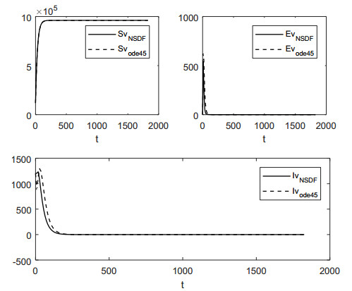
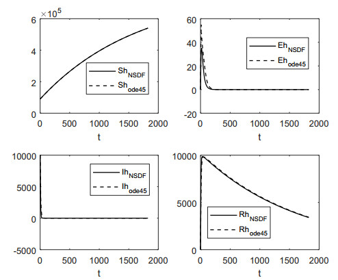
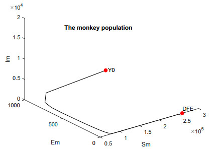
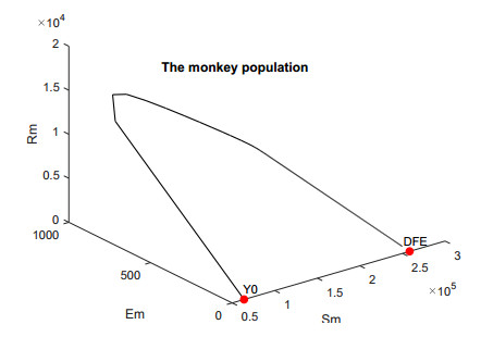
In this work, we investigate the transmission dynamics of the Zika virus, considering both a compartmental model involving humans and mosquitoes and an extended model that introduces a non-human primate (monkey) as a second reservoir host. The novelty of our approach lies in the later generalization of the model using a fractional time derivative. The significance of this study is underscored by its contribution to understanding the complex dynamics of Zika virus transmission. Unlike previous studies, we incorporate a non-human primate reservoir host into the model, providing a more comprehensive representation of the disease spread. Our results reveal the importance of utilizing a nonstandard finite difference (NSFD) scheme to simulate the disease's dynamics accurately. This NSFD scheme ensures the positivity of the solution and captures the correct asymptotic behavior, addressing a crucial limitation of standard solvers like the Runge-Kutta Fehlberg method (ode45). The numerical simulations vividly demonstrate the advantages of our approach, particularly in terms of positivity preservation, offering a more reliable depiction of Zika virus transmission dynamics. From these findings, we draw the conclusion that considering a non-human primate reservoir host and employing an NSFD scheme significantly enhances the accuracy and reliability of modeling Zika virus transmission. Researchers and policymakers can use these insights to develop more effective strategies for disease control and prevention.
- nonstandard finite difference scheme,
- positivity,
- Zika virus,
- compartment models,
- time-fractional models,
- epidemiology,
- SEIR model,
- human-vector models
Citation: Maghnia Hamou Maamar, Matthias Ehrhardt, Louiza Tabharit. A nonstandard finite difference scheme for a time-fractional model of Zika virus transmission[J]. Mathematical Biosciences and Engineering, 2024, 21(1): 924-962. doi: 10.3934/mbe.2024039

Related Papers:

Abstract

In this work, we investigate the transmission dynamics of the Zika virus, considering both a compartmental model involving humans and mosquitoes and an extended model that introduces a non-human primate (monkey) as a second reservoir host. The novelty of our approach lies in the later generalization of the model using a fractional time derivative. The significance of this study is underscored by its contribution to understanding the complex dynamics of Zika virus transmission. Unlike previous studies, we incorporate a non-human primate reservoir host into the model, providing a more comprehensive representation of the disease spread. Our results reveal the importance of utilizing a nonstandard finite difference (NSFD) scheme to simulate the disease's dynamics accurately. This NSFD scheme ensures the positivity of the solution and captures the correct asymptotic behavior, addressing a crucial limitation of standard solvers like the Runge-Kutta Fehlberg method (ode45). The numerical simulations vividly demonstrate the advantages of our approach, particularly in terms of positivity preservation, offering a more reliable depiction of Zika virus transmission dynamics. From these findings, we draw the conclusion that considering a non-human primate reservoir host and employing an NSFD scheme significantly enhances the accuracy and reliability of modeling Zika virus transmission. Researchers and policymakers can use these insights to develop more effective strategies for disease control and prevention.

References

[1]	G. W. Dick, S. F. Kitchen, A. J. Haddow, Zika virus. I. isolations and serological specificity, Trans. R. Soc. Trop. Med. Hyg., 46 (1952), 509–520. https://doi.org/10.1016/0035-9203(52)90042-4 doi: 10.1016/0035-9203(52)90042-4
[2]	G. W. Dick, S. F. Kitchen, A. J. Haddow, Zika virus. II. pathogenicity and physical properties, Trans. R. Soc. Trop. Med. Hyg., 46 (1952), 521–534. https://doi.org/10.1016/0035-9203(52)90043-6 doi: 10.1016/0035-9203(52)90043-6
[3]	M. R. Duffy, T. H. Chen, W. T. Hancock, A. M. Powers, J. L. Kool, R. S. Lanciotti, Zika virus outbreak on Yap Island, federated states of Micronesia, N. Engl. J. Med., 360 (2009), 2536–2543. https://doi.org/10.1056/NEJMoa0805715 doi: 10.1056/NEJMoa0805715
[4]	S. Ioos, H. P. Mallet, I. L. Goffart, V. Gauthier, T. Cardoso, M. Herida, Current Zika virus epidemiology and recent epidemics, Med. Mal. Infect., 44 (2014), 302–307. https://doi.org/10.1016/j.medmal.2014.04.008 doi: 10.1016/j.medmal.2014.04.008
[5]	V. M. C. Lormeau, C. Roche, A. Teissier, E. Robin, A. Berry, H. Mallet, et al., Zika virus, French Polynesia, South Pacific, 2013, Emerg. Infect. Dis., 20 (2014), 1085–1086. https://doi.org/10.3201/eid2006.140138
[6]	C. Zanluca, V. C. A. Melo, A. L. P. Mosimann, G. I. V. Santos, C. N. D. Santos, K. Luz, First report of autochthonous transmission of Zika virus in Brazil, Inst. Oswaldo Cruz., 110 (2015), 569–572. https://doi.org/10.1590/0074-02760150192 doi: 10.1590/0074-02760150192
[7]	D. Gatherer, A. Kohl, Zika virus: a previously slow pandemic spreads rapidly through the Americas, J. Gen. Virol., 97 (2016), 269–273. https://doi.org/10.1099/jgv.0.000381 doi: 10.1099/jgv.0.000381
[8]	J. P. Messina, M. Kraemer, O. J. Brady, D. M. Pigott, F. M. Shearer, D. J. Weiss, et al., Mapping global environmental suitability for Zika virus, elife, 5 (2016), e15272. https://doi.org/10.7554/eLife.15272 doi: 10.7554/eLife.15272
[9]	V. L. P. Junior, K. Luz, R. Parreira, P. Ferrinho, Zika virus: a review to clinicians, Acta Med. Port., 28 (2015), 760–765.
[10]	R. Becker, Missing link: Animal models to study whether Zika causes birth defects, Nat. Med., 22 (2016), 225–227. https://doi.org/10.1038/nm0316-225 doi: 10.1038/nm0316-225
[11]	L. Bouzid, O. Belhamiti, Effect of seasonal changes on predictive model of bovine babesiosis transmission, Int. J. Model. Simul. Sci. Comput., 8 (2017), 1–17. https://doi.org/10.1142/S1793962317500301 doi: 10.1142/S1793962317500301
[12]	E. B. Hayes, Zika virus outside Africa, Emerg. Infect. Dis. 15 (2009), 1347–1350. https://doi.org/10.3201/eid1509.090442
[13]	M. H. Maamar, L. Bouzid, O. Belhamiti, F. B. M. Belgacem, Stability and numerical study of theoretical model of Zika virus transmission, Int. J. Math. Modell. Numer. Optim., 10 (2020), 141–166. https://doi.org/10.1504/IJMMNO.2020.106528 doi: 10.1504/IJMMNO.2020.106528
[14]	F. L. H. Wertheim, P. Horby, J. P. Woodall, Atlas of Human Infectious Diseases, Wiley-Blackwell, Oxford, 2012.
[15]	W. O. Kermack, A. G. McKendrick, A contribution to the mathematical theory of epidemics, Proc. R. Soc. London, Ser. A, 115 (1927), 700–721. https://doi.org/10.1098/rspa.1927.0118 doi: 10.1098/rspa.1927.0118
[16]	C. Manore, M. Hyman, Mathematical models for fighting Zika virus, SIAM News, 49 (2016).
[17]	D. Gao, Y. Lou, D. He, T. C. Porco, Y. Kuang, G. Chowell, et al., Prevention and control of Zika as a mosquito-borne and sexually transmitted disease: a mathematical modeling analysis, Sci. Rep., 6 (2016), 28070. https://doi.org/10.1038/srep28070 doi: 10.1038/srep28070
[18]	E. K. Lee, Y. Liu, F. H. Pietz, A compartmental model for Zika virus with dynamic human and vector populations, AMIA Annu. Symp. Proc., 2016 (2011), 743–752.
[19]	H. Nishiura, R. Kinoshita, K. Mizumoto, Y. Yasuda, K. Nah, Transmission potential of Zika virus infection in the south pacific, Int. J. Infect. Dis., 45 (2016), 95–97. https://doi.org/10.1016/j.ijid.2016.02.017 doi: 10.1016/j.ijid.2016.02.017
[20]	S. Rezapour, H. Mohammadi, M. E. Samei, SEIR epidemic model for COVID-19 transmission by Caputo derivative of fractional order, Adv. Differ. Equations, 2020 (2020), 1–19. https://doi.org/10.1186/s13662-020-02952-y doi: 10.1186/s13662-020-02952-y
[21]	S. Ahmad, M. Rahman, M. Arfan, On the analysis of semi-analytical solutions of Hepatitis B epidemic model under the Caputo-Fabrizio operator, Chaos, Solitons Fractals, 146 (2021), 110892. https://doi.org/10.1016/j.chaos.2021.110892 doi: 10.1016/j.chaos.2021.110892
[22]	M. A. Taneco-Hernández, C. Vargas-De-León, Stability and Lyapunov functions for systems with Atangana-Baleanu Caputo derivative: an HIV/AIDS epidemic model, Chaos, Solitons Fractals, 132 (2020), 109586. https://doi.org/10.1016/j.chaos.2019.109586 doi: 10.1016/j.chaos.2019.109586
[23]	S. Qureshi, R. Jan, Modeling of measles epidemic with optimized fractional order under Caputo differential operator, Chaos, Solitons Fractals, 145 (2021), 110766. https://doi.org/10.1016/j.chaos.2021.110766 doi: 10.1016/j.chaos.2021.110766
[24]	W. Wang, M. Zhou, T. Zhang, Z. Feng, Dynamics of a Zika virus transmission model with seasonality and periodic delays, Commun. Nonl. Sci. Numer. Simul., 116 (2023), 106830. https://doi.org/10.1016/j.cnsns.2022.106830 doi: 10.1016/j.cnsns.2022.106830
[25]	M. A. Ibrahim, A. Dénes, A mathematical model for Zika Virus infection and microcephaly risk considering sexual and vertical transmission, Axioms, 12 (2023), 263. https://doi.org/10.3390/axioms12030263 doi: 10.3390/axioms12030263
[26]	M. Murugappan, R. Grienggarai, V. Govindan, Mathematical modelling on the transmission dynamics of Zika Virus, Int. J. Robot., Autom. Sci., 5 (2023), 79–84. https://doi.org/10.33093/ijoras.2023.5.2.9 doi: 10.33093/ijoras.2023.5.2.9
[27]	F. A. Oguntolu, O. J. Peter, A. Yusuf, B. I. Omede, G. Bolarin, T. A. Ayoola, Mathematical model and analysis of the soil-transmitted helminth infections with optimal control, Model. Earth Syst. Environm., 2023 (2023), 1–15. https://doi.org/10.1007/s40808-023-01815-1 doi: 10.1007/s40808-023-01815-1
[28]	O. J. Peter, H. S. Panigoro, A. Abidemi, M. M. Ojo, F.A. Oguntolu, Mathematical model of COVID-19 pandemic with double dose vaccination, Acta Biotheor., 71 (2023), 9. https://doi.org/10.1007/s10441-023-09460-y doi: 10.1007/s10441-023-09460-y
[29]	A. J. Kucharski, S. Funk, R. M. Eggo, H. P. Mallet, W. J. Edmunds, E. J. Nilles, Transmission dynamics of Zika virus in island populations: a modelling analysis of the 2013/14 French Polynesia outbreak, PLoS Negl. Trop. Dis., 10 (2016), e0004726. https://doi.org/10.1371/journal.pntd.0004726 doi: 10.1371/journal.pntd.0004726
[30]	J. P. T. Boorman, J. S. Porterfield, A simple technique for infection of mosquitoes with viruses, transmission of Zika virus, Trans. Roy. Soc. Trop. Med. Hyg., 50 (1956), 238–242. https://doi.org/10.1016/0035-9203(56)90029-3 doi: 10.1016/0035-9203(56)90029-3
[31]	M. Darwish, A seroepidemiological survey for bunyaviridae and certain other arboviruses in Pakistan, Trans. R. Soc. Trop. Med. Hyg., 77 (1983), 446–450. https://doi.org/10.1016/0035-9203(83)90108-6 doi: 10.1016/0035-9203(83)90108-6
[32]	C. Castillo-Chávez, H. Thieme, Asymptotically autonomous epidemic models, in Mathematical Population Dynamics: Analysis of Heterogeneity, Wuerz Publishing, Winnipeg, (1995), 33–50.
[33]	G. M. R. Costa, M. Lobosco, M. Ehrhardt, R. F. Reis, Mathematical analysis and a nonstandard scheme for a model of the immune response against COVID-19, in Mathematical and Computational Modeling of Phenomena Arising in Population Biology and Nonlinear Oscillations: In honour of the 80th birthday of Ronald E. Mickens, AMS Contemporary Mathematics, 2023.
[34]	K. Diethelm, A fractional calculus based model for the simulation of an outbreak of Dengue fever, Nonl. Dyn., 71 (2013), 613–619. https://doi.org/10.1007/s11071-012-0475-2 doi: 10.1007/s11071-012-0475-2
[35]	H. K. Khalil, Nonlinear Systems, Prentice-Hall, London, UK, 1996.
[36]	R. Gorenflo, A. A. Kilbas, F. Mainardi, S. V. Rogosin, Mittag-Leffler Functions, Related Topics and Applications, Springer, Berlin-Heidelberg, 2014.
[37]	C. Vargas-De-León, Volterra-type Lyapunov functions for fractional-order epidemic systems, Commun. Nonl. Sci. Numer. Simul., 24 (2015), 75–85. https://doi.org/10.1016/j.cnsns.2014.12.013 doi: 10.1016/j.cnsns.2014.12.013
[38]	R. E. Mickens, Applications of Nonstandard Finite Difference Schemes, World Scientific, 2000.
[39]	M. M. Khalsaraei, Positivity of an explicit Runge–Kutta method, Ain Shams Eng. J., 6 (2015), 1217–1223. https://doi.org/10.1016/j.asej.2015.05.018 doi: 10.1016/j.asej.2015.05.018
[40]	A. Gerisch, R. Weiner, The positivity of low-order explicit Runge-Kutta schemes applied in splitting methods, Comput. Math. Appl., 45 (2003), 53–67. https://doi.org/10.1016/S0898-1221(03)80007-X doi: 10.1016/S0898-1221(03)80007-X
[41]	R. E. Mickens, Calculation of denominator functions for nonstandard finite difference schemes for differential equations satisfying a positivity condition, Numer. Methods Partial Differ. Equations, 23 (2007), 672–691. https://doi.org/10.1002/num.20198 doi: 10.1002/num.20198
[42]	S. Berkhahn, M. Ehrhardt, A physics-informed neural network to model COVID-19 infection and hospitalization scenarios, Adv. Contin. Discrete Models, 2022 (2022), 61. https://doi.org/10.1186/s13662-022-03733-5 doi: 10.1186/s13662-022-03733-5
[43]	S. Treibert, H. Brunner, M. Ehrhardt, A nonstandard finite difference scheme for the SVICDR model to predict COVID-19 dynamics, Math. Biosci. Eng., 19 (2022), 1213–1238. https://doi.org/10.3934/mbe.2022056 doi: 10.3934/mbe.2022056
[44]	M. Ehrhardt, R. E. Mickens, A Nonstandard Finite Difference Scheme for Solving a Zika Virus Model, unpublished manuscript, 2017.
[45]	D. Matignon, Stability results for fractional differential equations with applications to control processing, Comput. Eng. Syst. Appl., 2 (1996), 963–968.
[46]	A. Ali, S. Islam, M. R. Khan, S. Rasheed, F. M. Allehiany, J. Baili, et al., Dynamics of a fractional order Zika virus model with mutant, Alexandria Eng. J., 61 (2022), 4821–4836. https://doi.org/10.1016/j.aej.2021.10.031 doi: 10.1016/j.aej.2021.10.031
[47]	A. Ali, F. S. Alshammari, S. Islam, M. A. Khan, S. Ullah, Modeling and analysis of the dynamics of novel coronavirus (COVID-19) with Caputo fractional derivative, Res. Phys., 20 (2021), 103669. https://doi.org/10.1016/j.rinp.2020.103669 doi: 10.1016/j.rinp.2020.103669

Reader Comments

Your name:*

Email:*
© 2024 the Author(s), licensee AIMS Press. This is an open access article distributed under the terms of the Creative Commons Attribution License (http://creativecommons.org/licenses/by/4.0)