4mCPred-GSIMP: Predicting DNA N4-methylcytosine sites in the mouse genome with multi-Scale adaptive features extraction and fusion

Jianhua Jia; Yu Deng; Mengyue Yi; Yuhui Zhu; Jianhua Jia; Yu Deng; Mengyue Yi; Yuhui Zhu

doi:10.3934/mbe.2024012

Mathematical Biosciences and Engineering

2024, Volume 21, Issue 1: 253-271. doi: 10.3934/mbe.2024012

Previous Article Next Article

Research article Special Issues

4mCPred-GSIMP: Predicting DNA N4-methylcytosine sites in the mouse genome with multi-Scale adaptive features extraction and fusion

School of Information Engineering, Jingdezhen Ceramic University, Jingdezhen 333403, China

Academic Editor: Qianqian Song

Received: 12 October 2023 Revised: 30 November 2023 Accepted: 04 December 2023 Published: 12 December 2023

The epigenetic modification of DNA N4-methylcytosine (4mC) is vital for controlling DNA replication and expression. It is crucial to pinpoint 4mC's location to comprehend its role in physiological and pathological processes. However, accurate 4mC detection is difficult to achieve due to technical constraints. In this paper, we propose a deep learning-based approach 4mCPred-GSIMP for predicting 4mC sites in the mouse genome. The approach encodes DNA sequences using four feature encoding methods and combines multi-scale convolution and improved selective kernel convolution to adaptively extract and fuse features from different scales, thereby improving feature representation and optimization effect. In addition, we also use convolutional residual connections, global response normalization and pointwise convolution techniques to optimize the model. On the independent test dataset, 4mCPred-GSIMP shows high sensitivity, specificity, accuracy, Matthews correlation coefficient and area under the curve, which are 0.7812, 0.9312, 0.8562, 0.7207 and 0.9233, respectively. Various experiments demonstrate that 4mCPred-GSIMP outperforms existing prediction tools.
- DNA N4-methylcytosine,
- multi-scale convolution,
- selective kernel convolution,
- global response normalization
Citation: Jianhua Jia, Yu Deng, Mengyue Yi, Yuhui Zhu. 4mCPred-GSIMP: Predicting DNA N4-methylcytosine sites in the mouse genome with multi-Scale adaptive features extraction and fusion[J]. Mathematical Biosciences and Engineering, 2024, 21(1): 253-271. doi: 10.3934/mbe.2024012

Related Papers:

Abstract

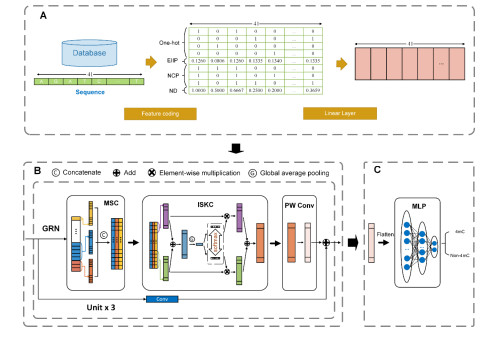
The epigenetic modification of DNA N4-methylcytosine (4mC) is vital for controlling DNA replication and expression. It is crucial to pinpoint 4mC's location to comprehend its role in physiological and pathological processes. However, accurate 4mC detection is difficult to achieve due to technical constraints. In this paper, we propose a deep learning-based approach 4mCPred-GSIMP for predicting 4mC sites in the mouse genome. The approach encodes DNA sequences using four feature encoding methods and combines multi-scale convolution and improved selective kernel convolution to adaptively extract and fuse features from different scales, thereby improving feature representation and optimization effect. In addition, we also use convolutional residual connections, global response normalization and pointwise convolution techniques to optimize the model. On the independent test dataset, 4mCPred-GSIMP shows high sensitivity, specificity, accuracy, Matthews correlation coefficient and area under the curve, which are 0.7812, 0.9312, 0.8562, 0.7207 and 0.9233, respectively. Various experiments demonstrate that 4mCPred-GSIMP outperforms existing prediction tools.

References

[1]	L. Zhao, J. Song, Y. Liu, C. Song, C. Yi, Mapping the epigenetic modifications of DNA and RNA, Protein Cell, 11 (2020), 792–808. https://doi.org/10.1007/s13238-020-00733-7 doi: 10.1007/s13238-020-00733-7
[2]	L. D. Moore, T. Le, G. Fan, DNA methylation and its basic function, Neuropsychopharmacology, 38 (2013), 23–38. https://doi.org/10.1038/npp.2012.112 doi: 10.1038/npp.2012.112
[3]	N. Zhang, C. Lin, X. Huang, A. Kolbanovskiy, B. E. Hingerty, S. Amin, et al., Methylation of cytosine at C5 in a CpG sequence context causes a conformational switch of a benzo[a]pyrene diol epoxide-N²-guanine adduct in DNA from a minor groove alignment to intercalation with base displacement, J. Mol. Biol., 346 (2005), 951–965. https://doi.org/10.1016/j.jmb.2004.12.027 doi: 10.1016/j.jmb.2004.12.027
[4]	A. Breiling, F. Lyko, Epigenetic regulatory functions of DNA modifications: 5-methylcytosine and beyond, Epigenet. Chromatin, 8 (2015), 24. https://doi.org/10.1186/s13072-015-0016-6 doi: 10.1186/s13072-015-0016-6
[5]	A. Jeltsch, R. Z. Jurkowska, New concepts in DNA methylation, Trends Biochem. Sci., 39 (2014), 310–318. https://doi.org/10.1016/j.tibs.2014.05.002 doi: 10.1016/j.tibs.2014.05.002
[6]	D. Schübeler, Function and information content of DNA methylation, Nature, 517 (2015), 321–326. https://doi.org/10.1038/nature14192 doi: 10.1038/nature14192
[7]	N. P. Blackledge, R. Klose, CpG island chromatin, Epigenetics, 6 (2011), 147–152. https://doi.org/10.4161/epi.6.2.13640 doi: 10.4161/epi.6.2.13640
[8]	F. J. Clasen, R. E. Pierneef, B. Slippers, O. Reva, EuGI: a novel resource for studying genomic islands to facilitate horizontal gene transfer detection in eukaryotes, BMC Genomics, 19 (2018). https://doi.org/10.1186/s12864-018-4724-8 doi: 10.1186/s12864-018-4724-8
[9]	X. Guo, Y. Guo, H. Chen, X. Liu, P. He, W. Li, et al., Systematic comparison of genome information processing and boundary recognition tools used for genomic island detection, Comput. Biol. Med., 166 (2023), 107550. https://doi.org/10.1016/j.compbiomed.2023.107550 doi: 10.1016/j.compbiomed.2023.107550
[10]	Q. Dai, C. Bao, Y. Hai, S. Ma, T. Zhou, C. Wang, et al., MTGIpick allows robust identification of genomic islands from a single genome, Briefings Bioinf., 19 (2018), 361–373. https://doi.org/10.1093/bib/bbw118 doi: 10.1093/bib/bbw118
[11]	A. Chialastri, S. Sarkar, E. E. Schauer, S. Lamba, S. S. Dey, Combinatorial quantification of 5mC and 5hmC at individual CpG dyads and the transcriptome in single cells reveals modulators of DNA methylation maintenance fidelity, preprint.
[12]	G. Luo, M. A. Blanco, E. L. Greer, C. He, Y. Shi, DNA N⁶-methyladenine: a new epigenetic mark in eukaryotes?, Nat. Rev. Mol. Cell Biol., 16 (2015), 705–710. https://doi.org/10.1038/nrm4076 doi: 10.1038/nrm4076
[13]	J. Beaulaurier, E. E. Schadt, G. Fang, Deciphering bacterial epigenomes using modern sequencing technologies, Nat. Rev. Genet., 20 (2019), 157–172. https://doi.org/10.1038/s41576-018-0081-3 doi: 10.1038/s41576-018-0081-3
[14]	M. Ehrlich, G. G. Wilson, K. C. Kuo, C. W. Gehrke, N4-methylcytosine as a minor base in bacterial DNA, Journal of Bacteriology, 169 (1987), 939–943. https://doi.org/10.1128/jb.169.3.939-943.1987 doi: 10.1128/jb.169.3.939-943.1987
[15]	F. Rodriguez, I. A. Yushenova, D. DiCorpo, I. R. Arkhipova, Bacterial N4-methylcytosine as an epigenetic mark in eukaryotic DNA, Nat. Commun., 13 (2022), 1072. https://doi.org/10.1038/s41467-022-28471-w doi: 10.1038/s41467-022-28471-w
[16]	M. Yu, L. Ji, D. A. Neumann, D. Chung, J. Groom, J. Westpheling, et al., Base-resolution detection of N 4-methylcytosine in genomic DNA using 4mC-Tet-assisted-bisulfite- sequencing, Nucleic Acids Res., 43 (2015), 148. https://doi.org/10.1093/nar/gkv738 doi: 10.1093/nar/gkv738
[17]	S. Ardui, A. Ameur, J. R. Vermeesch, M. S. Hestand, Single molecule real-time (SMRT) sequencing comes of age: applications and utilities for medical diagnostics, Nucleic Acids Res., 46 (2018), 2159–2168. https://doi.org/10.1093/nar/gky066 doi: 10.1093/nar/gky066
[18]	B. Manavalan, S. Basith, T. H. Shin, D. Y. Lee, L. Wei, G. Lee, 4mCpred-EL: An ensemble learning framework for identification of DNA N4-methylcytosine sites in the mouse genome, Cells, 8 (2019), 1332. https://doi.org/10.3390/cells8111332 doi: 10.3390/cells8111332
[19]	W. He, C. Jia, Q. Zou, 4mCPred: machine learning methods for DNA N⁴-methylcytosine sites prediction, Bioinformatics, 35 (2019), 593–601. https://doi.org/10.1093/bioinformatics/bty668 doi: 10.1093/bioinformatics/bty668
[20]	M. M. Hasan, B. Manavalan, W. Shoombuatong, M. S. Khatun, H. Kurata, i4mC-Mouse: Improved identification of DNA N4-methylcytosine sites in the mouse genome using multiple encoding schemes, Comput. Struct. Biotechnol. J., 18 (2020), 906–912. https://doi.org/10.1016/j.csbj.2020.04.001 doi: 10.1016/j.csbj.2020.04.001
[21]	W. Chen, H. Yang, P. Feng, H. Ding, H. Lin, iDNA4mC: identifying DNA N⁴-methylcytosine sites based on nucleotide chemical properties, Bioinformatics, 33 (2017), 3518–3523. https://doi.org/10.1093/bioinformatics/btx479 doi: 10.1093/bioinformatics/btx479
[22]	B. Manavalan, S. Basith, T. H. Shin, L. Wei, G. Lee, Meta-4mCpred: A sequence-based meta-predictor for accurate DNA 4mC site prediction using effective feature representation, Mol. Ther.-Nucleic Acids, 16 (2019), 733–744. https://doi.org/10.1016/j.omtn.2019.04.019 doi: 10.1016/j.omtn.2019.04.019
[23]	H. Xu, P. Jia, Z. Zhao, Deep4mC: systematic assessment and computational prediction for DNA N4-methylcytosine sites by deep learning, Briefings Bioinf., 22 (2021). https://doi.org/10.1093/bib/bbaa099 doi: 10.1093/bib/bbaa099
[24]	Q. Liu, J. Chen, Y. Wang, S. Li, C. Jia, J. Song, et al., DeepTorrent: a deep learning-based approach for predicting DNA N4-methylcytosine sites, Briefings Bioinf., 22 (2021). https://doi.org/10.1093/bib/bbaa124 doi: 10.1093/bib/bbaa124
[25]	X. Yu, J. Ren, Y. Cui, R. Zeng, H. Long, C. Ma, DRSN4mCPred: accurately predicting sites of DNA N4-methylcytosine using deep residual shrinkage network for diagnosis and treatment of gastrointestinal cancer in the precision medicine era, Front. Med., 10 (2023). https://doi.org/10.3389/fmed.2023.1187430 doi: 10.3389/fmed.2023.1187430
[26]	Y. Yu, W. He, J. Jin, G. Xiao, L. Cui, R. Zeng, et al., iDNA-ABT: advanced deep learning model for detecting DNA methylation with adaptive features and transductive information maximization, Bioinformatics, 37 (2021), 4603–4610. https://doi.org/10.1093/bioinformatics/btab677 doi: 10.1093/bioinformatics/btab677
[27]	J. Jin, Y. Yu, R. Wang, X. Zeng, C. Pang, Y. Jiang, et al., iDNA-ABF: multi-scale deep biological language learning model for the interpretable prediction of DNA methylations, Genome Biol., 23 (2022). https://doi.org/10.1186/s13059-022-02780-1 doi: 10.1186/s13059-022-02780-1
[28]	W. Zeng, A. Gautam, D. H. Huson, MuLan-Methyl-multiple transformer-based language models for accurate DNA methylation prediction, GigaScience, 12 (2023). https://doi.org/10.1093/gigascience/giad054 doi: 10.1093/gigascience/giad054
[29]	M. U. Rehman, H. Tayara, K. T. Chong, DCNN-4mC: Densely connected neural network based N4-methylcytosine site prediction in multiple species, Comput. Struct. Biotechnol. J., 19 (2021), 6009–6019. https://doi.org/10.1016/j.csbj.2021.10.034 doi: 10.1016/j.csbj.2021.10.034
[30]	S. Park, M. U. Rehman, F. Ullah, H. Tayara, K. T. Chong, I. Birol, iCpG-Pos: an accurate computational approach for identification of CpG sites using positional features on single-cell whole genome sequence data, Bioinformatics, 39 (2023). https://doi.org/10.1093/bioinformatics/btad474 doi: 10.1093/bioinformatics/btad474
[31]	L. Zhang, X. Xiao, Z. Xu, iPromoter-5mC: A novel fusion decision predictor for the identification of 5-Methylcytosine sites in genome-Wide DNA promoters, Front. Cell Dev. Biol., 8 (2020). https://doi.org/10.3389/fcell.2020.00614 doi: 10.3389/fcell.2020.00614
[32]	D. Y. Lim, M. U. Rehman, K. T. Chong, iRG-4mC: Neural network based tool for identification of DNA 4mC sites in rosaceae genome, Symmetry, 13 (2021), 899. https://doi.org/10.3390/sym13050899 doi: 10.3390/sym13050899
[33]	M. U. Rehman, K. J. Hong, H. Tayara, K. T. Chong, m6A-NeuralTool: Convolution neural tool for RNA N6-Methyladenosine site identification in different species, IEEE Access, 9 (2021), 17779–17786. https://doi.org/10.1109/access.2021.3054361 doi: 10.1109/access.2021.3054361
[34]	Q. H. Nguyen, H. V. Tran, B. P. Nguyen, T. T. T. Do, Identifying transcription factors that prefer binding to methylated DNA using reduced G-Gap dipeptide composition, ACS Omega, 7 (2022), 32322–32330. https://doi.org/10.1021/acsomega.2c03696 doi: 10.1021/acsomega.2c03696
[35]	Z. Li, H. Jiang, L. Kong, Y. Chen, K. Lang, X. Fan, et al., Deep6mA: A deep learning framework for exploring similar patterns in DNA N6-methyladenine sites across different species, PLOS Comput. Biol., 17 (2021), 1008767. https://doi.org/10.1371/journal.pcbi.1008767 doi: 10.1371/journal.pcbi.1008767
[36]	X. Cheng, J. Wang, Q. Li, T. Liu, BiLSTM-5mC: A bidirectional long short-term memory-based approach for predicting 5-Methylcytosine sites in genome-wide DNA promoters, Molecules, 26 (2021), 7414. https://doi.org/10.3390/molecules26247414 doi: 10.3390/molecules26247414
[37]	Z. Abbas, H. Tayara, K. T. Chong, 4mCPred-CNN-Prediction of DNA N4-Methylcytosine in the mouse genome using a convolutional neural network, Genes, 12 (2021), 296. https://doi.org/10.3390/genes12020296 doi: 10.3390/genes12020296
[38]	J. Jin, Y. Yu, L. Wei, Mouse4mC-BGRU: Deep learning for predicting DNA N4-methylcytosine sites in mouse genome, Methods, 204 (2022), 258–262. https://doi.org/10.1016/j.ymeth.2022.01.009 doi: 10.1016/j.ymeth.2022.01.009
[39]	P. Zheng, G. Zhang, Y. Liu, G. Huang, MultiScale-CNN-4mCPred: a multi-scale CNN and adaptive embedding-based method for mouse genome DNA N4-methylcytosine prediction, BMC Bioinformatics, 24 (2023). https://doi.org/10.1186/s12859-023-05135-0 doi: 10.1186/s12859-023-05135-0
[40]	T. Nguyen-Vo, Q. H. Trinh, L. Nguyen, P. Nguyen-Hoang, S. Rahardja, B. P. Nguyen, i4mC-GRU: Identifying DNA N4-Methylcytosine sites in mouse genomes using bidirectional gated recurrent unit and sequence-embedded features, Comput. Struct. Biotechnol. J., 21 (2023), 3045–3053. https://doi.org/10.1016/j.csbj.2023.05.014 doi: 10.1016/j.csbj.2023.05.014
[41]	C. Szegedy, W. Liu, Y. Jia, P. Sermanet, S. Reed, D. Anguelov, et al., Going deeper with convolutions, in 2015 IEEE Conference on Computer Vision and Pattern Recognition (CVPR), IEEE, (2015), 1–9. https://doi.org/10.1109/CVPR.2015.7298594
[42]	X. Li, W. Wang, X. Hu, J. Yang, Selective kernel networks, in 2019 IEEE/CVF Conference on Computer Vision and Pattern Recognition (CVPR), (2019), 510–519. https://doi.org/10.1109/CVPR.2019.00060
[43]	S. Woo, S. Debnath, R. Hu, X. Chen, Z. Liu, I. S. Kweon, et al., ConvNeXt V2: Co-Designing and scaling ConvNets with masked autoencoders, in 2023 IEEE/CVF Conference on Computer Vision and Pattern Recognition (CVPR), (2023), 16133–16142. https://doi.org/10.1109/CVPR52729.2023.01548
[44]	A. G. Howard, M. Zhu, B. Chen, D. Kalenichenko, W. Wang, T. Weyand, et al., MobileNets: efficient convolutional neural networks for mobile vision applications, preprint, arXiv: 1704.04861.
[45]	P. Ye, Y. Luan, K. Chen, Y. Liu, C. Xiao, Z. Xie, MethSMRT: an integrative database for DNA N6-methyladenine and N4-methylcytosine generated by single-molecular real-time sequencing, Nucleic Acids Res., 45 (2017), 85–89. https://doi.org/10.1093/nar/gkw950 doi: 10.1093/nar/gkw950
[46]	L. Fu, B. Niu, Z. Zhu, S. Wu, W. Li, CD-HIT: accelerated for clustering the next-generation sequencing data, Bioinformatics, 28 (2012), 3150–3152. https://doi.org/10.1093/bioinformatics/bts565 doi: 10.1093/bioinformatics/bts565
[47]	W. Chen, H. Tang, J. Ye, H. Lin, K. Chou, iRNA-PseU: Identifying RNA pseudouridine sites, Mol. Ther.-Nucleic Acids, 5 (2016), 332.
[48]	T. Nguyen-Vo, Q. H. Nguyen, T. T. T. Do, T. Nguyen, S. Rahardja, B. P. Nguyen, iPseU-NCP: Identifying RNA pseudouridine sites using random forest and NCP-encoded features, BMC Genomics, 20 (2019). https://doi.org/10.1186/s12864-019-6357-y doi: 10.1186/s12864-019-6357-y
[49]	A. S. Nair, S. P. Sreenadhan, A coding measure scheme employing electron-ion interaction pseudopotential (EⅡP), Bioinformation, 1 (2006), 197–202.
[50]	R. Avenash, P. Viswanath, Semantic segmentation of satellite images using a modified CNN with hard-swish activation function, in Proceedings of the 14th International Joint Conference on Computer Vision, Imaging and Computer Graphics Theory and Applications, (2019), 413–420.
[51]	K. He, X. Zhang, S. Ren, J. Sun, Deep residual learning for image recognition, in 2016 IEEE Conference on Computer Vision and Pattern Recognition (CVPR), (2016), 770–778. https://doi.org/10.1109/CVPR.2016.90
[52]	A. Krizhevsky, I. Sutskever, G. E. Hinton, ImageNet classification with deep convolutional neural networks, Commun. ACM, 60 (2017), 84–90. https://doi.org/10.1145/3065386 doi: 10.1145/3065386
[53]	S. Ioffe, C. Szegedy, Batch normalization: Accelerating deep network training by reducing internal covariate shift, preprint, arXiv: 1502.03167.
[54]	J. L. Ba, J. R. Kiros, G. E. Hinton, Layer normalization, preprint, arXiv: 1607.06450.
[55]	M. Sokolova, G. Lapalme, A systematic analysis of performance measures for classification tasks, Inf. Process. Manage., 45 (2009), 427–437. https://doi.org/10.1016/j.ipm.2009.03.002 doi: 10.1016/j.ipm.2009.03.002
[56]	H. Lv, F. Dao, D. Zhang, Z. Guan, H. Yang, W. Su, et al., iDNA-MS: An integrated computational tool for detecting DNA modification sites in multiple genomes, iScience, 23 (2020), 100991. https://doi.org/10.1016/j.isci.2020.100991 doi: 10.1016/j.isci.2020.100991
[57]	A. Vaswani, N. Shazeer, N. Parmar, J. Uszkoreit, L. Jones, A. N. Gomez, et al., Attention is all you need, preprint, arXiv: 1706.03762v5.

Reader Comments

Your name:*

Email:*
© 2024 the Author(s), licensee AIMS Press. This is an open access article distributed under the terms of the Creative Commons Attribution License (http://creativecommons.org/licenses/by/4.0)