Research on bearing fault diagnosis based on a multimodal method

Hao Chen; Shengjie Li; Xi Lu; Qiong Zhang; Jixining Zhu; Jiaxin Lu; Hao Chen; Shengjie Li; Xi Lu; Qiong Zhang; Jixining Zhu; Jiaxin Lu

doi:10.3934/mbe.2024338

Mathematical Biosciences and Engineering

2024, Volume 21, Issue 12: 7688-7706. doi: 10.3934/mbe.2024338

Previous Article Next Article

Research article

Research on bearing fault diagnosis based on a multimodal method

1.
School of Information Engineering, Nantong Institute of Technology, Nantong 226002, Jiangsu, China
2.
Division of Information and Communication Convergence Engineering, Mokwon University, Daejeon 35349, Korea

Received: 17 September 2024 Revised: 16 November 2024 Accepted: 22 November 2024 Published: 04 December 2024

As an essential component of mechanical systems, bearing fault diagnosis is crucial to ensure the safe operation of the equipment. However, vibration data from bearings often exhibit non-stationary and nonlinear features, which complicates fault diagnosis. To address this challenge, this paper introduces a novel multi-scale time-frequency and statistical features fusion model (MTSF-FM). Specifically, the method first employs continuous wavelet transform to generate time-frequency images, capturing local and global features of the signal at different scales. Contrast enhancement techniques are then used to improve the visual quality of these images. Next, features are extracted from the time-frequency images using a visual geometry group network to obtain deep features of image modalities. In parallel, 13 key features are extracted from the original vibration data in the time-frequency domain. Convolutional neural networks are then employed for deep feature extraction. Experimental results demonstrate that MTSF-FM achieves accuracies of 98.5% and 95.1% on two public datasets. These findings highlight the effectiveness of MTSF-FM in analyzing complex vibration data and propose a novel method for bearing fault diagnosis.
- bearing fault diagnosis,
- non-stationary,
- nonlinear,
- time-frequency,
- deep feature
Citation: Hao Chen, Shengjie Li, Xi Lu, Qiong Zhang, Jixining Zhu, Jiaxin Lu. Research on bearing fault diagnosis based on a multimodal method[J]. Mathematical Biosciences and Engineering, 2024, 21(12): 7688-7706. doi: 10.3934/mbe.2024338

Related Papers:

Abstract

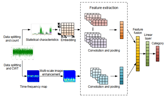
As an essential component of mechanical systems, bearing fault diagnosis is crucial to ensure the safe operation of the equipment. However, vibration data from bearings often exhibit non-stationary and nonlinear features, which complicates fault diagnosis. To address this challenge, this paper introduces a novel multi-scale time-frequency and statistical features fusion model (MTSF-FM). Specifically, the method first employs continuous wavelet transform to generate time-frequency images, capturing local and global features of the signal at different scales. Contrast enhancement techniques are then used to improve the visual quality of these images. Next, features are extracted from the time-frequency images using a visual geometry group network to obtain deep features of image modalities. In parallel, 13 key features are extracted from the original vibration data in the time-frequency domain. Convolutional neural networks are then employed for deep feature extraction. Experimental results demonstrate that MTSF-FM achieves accuracies of 98.5% and 95.1% on two public datasets. These findings highlight the effectiveness of MTSF-FM in analyzing complex vibration data and propose a novel method for bearing fault diagnosis.

References

[1]	C. Li, S. Li, Y. Feng, K. Gryllias, F. Gu, M. Pecht, Small data challenges for intelligent prognostics and health management: A review, Artif. Intell. Rev., 57 (2024), 214. https://doi.org/10.1007/s10462-024-10820-4 doi: 10.1007/s10462-024-10820-4
[2]	X. Chen, R. Yang, Y. Xue, M. Huang, R. Ferrero, Z. Wang, Deep transfer learning for bearing fault diagnosis: A systematic review since 2016, IEEE Trans. Instrum. Meas., 72 (2023), 1–21. https://doi.org/10.1109/TIM.2023.3244237 doi: 10.1109/TIM.2023.3244237
[3]	G. J. Jang, M. C. Noh, S. S. Kim, C. S. Shin, S. S. Lee, C. J. Lee, Vibration data feature extraction and deep learning-based preprocessing method for highly accurate motor fault diagnosis, J. Comput. Des. Eng., 10 (2023), 204–220. https://doi.org/10.1093/jcde/qwac128 doi: 10.1093/jcde/qwac128
[4]	Y. Xue, C. Wen, Z. Wang, W. Liu, G. Chen, A novel framework for motor bearing fault diagnosis based on multi-transformation domain and multi-source data, Knowledge-Based Syst., 283 (2024), 111205. https://doi.org/10.1016/j.knosys.2023.111205 doi: 10.1016/j.knosys.2023.111205
[5]	M. Sohaib, M. J. Kim, Fault diagnosis of rotary machine bearings under inconsistent working conditions, IEEE Trans. Instrum. Meas., 69 (2019), 3334–3347. https://doi.org/10.1109/TIM.2019.2933342 doi: 10.1109/TIM.2019.2933342
[6]	J. Pacheco-Chérrez, A. J. Fortoul-Díaz, F. Cortés-Santacruz, M. L. Aloso-Valerdi, I. D. Ibarra-Zarate, Bearing fault detection with vibration and acoustic signals: Comparison among different machine leaning classification methods, Eng. Fail. Anal., 139 (2022), 106515. https://doi.org/10.1016/j.engfailanal.2022.106515 doi: 10.1016/j.engfailanal.2022.106515
[7]	J. Jiao, M. Zhao, J. Lin, K. Liang, A comprehensive review on convolutional neural network in machine fault diagnosis, Neurocomputing, 417 (2020), 36–63. https://doi.org/10.1016/j.neucom.2020.07.088 doi: 10.1016/j.neucom.2020.07.088
[8]	H. Wang, Z. Liu, D. Peng, Z. Cheng, Attention-guided joint learning CNN with noise robustness for bearing fault diagnosis and vibration signal denoising, ISA Trans., 128 (2022), 470–484. https://doi.org/10.1016/j.isatra.2021.11.028 doi: 10.1016/j.isatra.2021.11.028
[9]	N. Liu, T. Schumacher, Y. Li, L. Xu, B. Wang, Damage detection in reinforced concrete member using local time-frequency transform applied to vibration measurements, Buildings, 13 (2023), 148. https://doi.org/10.3390/buildings13010148 doi: 10.3390/buildings13010148
[10]	P. Zhou, S. Chen, Q. He, D. Wang, Z. Peng, Rotating machinery fault-induced vibration signal modulation effects: A review with mechanisms, extraction methods and applications for diagnosis, Mech. Syst. Signal Process., 200 (2023), 110489. https://doi.org/10.1016/j.ymssp.2023.110489 doi: 10.1016/j.ymssp.2023.110489
[11]	H. Tao, J. Qiu, Y. Chen, V. Stojanovic, L. Cheng, Unsupervised cross-domain rolling bearing fault diagnosis based on time-frequency information fusion, J. Franklin Inst., 360 (2023), 1454–1477. https://doi.org/10.1016/j.jfranklin.2022.11.004 doi: 10.1016/j.jfranklin.2022.11.004
[12]	C. Che, H. Wang, X. Ni, Q. Fu, Domain adaptive deep belief network for rolling bearing fault diagnosis, Comput. Ind. Eng., 143 (2020), 106427. https://doi.org/10.1016/j.cie.2020.106427 doi: 10.1016/j.cie.2020.106427
[13]	K. Berahmand, F. Daneshfar, E. S. Salehi, Y. Li, Y. Xu, Autoencoders and their applications in machine learning: A survey, Artif. Intell. Rev., 57 (2024), 28. https://doi.org/10.1007/s10462-023-10662-6 doi: 10.1007/s10462-023-10662-6
[14]	S. Abdollahi, A. Deldari, H. Asadi, A. Montazerolghaem, S. M. Mazinani, Flow-aware forwarding in SDN datacenters using a knapsack-PSO-based solution, IEEE Trans. Netw. Serv. Manage., 18 (2021), 2902–2914. https://doi.org/10.1109/TNSM.2021.3064974 doi: 10.1109/TNSM.2021.3064974
[15]	S. Shen, H. Lu, M. Sadoughi, C. Hu, V. Nemani, A. Thelen, et al., A physics-informed deep learning approach for bearing fault detection, Eng. Appl. Artif. Intell., 103 (2021), 104295. https://doi.org/10.1016/j.engappai.2021.104295 doi: 10.1016/j.engappai.2021.104295
[16]	A. Khorram, M. Khalooei, M. Rezghi, End-to-end CNN+ LSTM deep learning approach for bearing fault diagnosis, Appl. Intell., 51 (2021), 736–751. https://doi.org/10.1007/s10489-020-01859-1 doi: 10.1007/s10489-020-01859-1
[17]	Y. Zou, Y. Zhang, H. Mao, Fault diagnosis on the bearing of traction motor in high-speed trains based on deep learning, Alexandria Eng. J., 60 (2021), 1209–1219. https://doi.org/10.1016/j.aej.2020.10.044 doi: 10.1016/j.aej.2020.10.044
[18]	R. Zhu, Y. Chen, W. Peng, S. Z. Ye, Bayesian deep-learning for RUL prediction: An active learning perspective, Reliab. Eng. Syst. Saf., 228 (2022), 108758. https://doi.org/10.1016/j.ress.2022.108758 doi: 10.1016/j.ress.2022.108758
[19]	Q. Janssens, V. Slavkovikj, B. Vervisch, K. Stockman, M. Loccufier, S. Verstockt, et al., Convolutional neural network based fault detection for rotating machinery, J. Sound Vib., 377 (2016), 331–345. https://doi.org/10.1016/j.jsv.2016.05.027 doi: 10.1016/j.jsv.2016.05.027
[20]	D. Ruan, J. Wang, J. Yan, C. Gühmann, CNN parameter design based on fault signal analysis and its application in bearing fault diagnosis, Adv. Eng. Inf., 55 (2023), 101877. https://doi.org/10.1016/j.aei.2023.101877 doi: 10.1016/j.aei.2023.101877
[21]	L. Jia, W. T. Chow, Y. Yuan, GTFE-Net: A gramian time frequency enhancement CNN for bearing fault diagnosis, Eng. Appl. Artif. Intell., 119 (2023), 105794. https://doi.org/10.1016/j.engappai.2022.105794 doi: 10.1016/j.engappai.2022.105794
[22]	Y. Hou, J. Wang, Z. Chen, J. Ma, T. Li, Diagnosisformer: An efficient rolling bearing fault diagnosis method based on improved Transformer, Eng. Appl. Artif. Intell., 124 (2023), 106507. https://doi.org/10.1016/j.engappai.2023.106507 doi: 10.1016/j.engappai.2023.106507
[23]	A. Choudhary, T. Mian, S. Fatima, Convolutional neural network based bearing fault diagnosis of rotating machine using thermal images, Measurement, 176 (2021), 109196. https://doi.org/10.1016/j.measurement.2021.109196 doi: 10.1016/j.measurement.2021.109196
[24]	X. Chen, B. Zhang, D. Gao, Bearing fault diagnosis base on multi-scale CNN and LSTM model, J. Intell. Manuf., 32 (2021), 971–987. https://doi.org/10.1007/s10845-020-01600-2 doi: 10.1007/s10845-020-01600-2
[25]	T. Han, L. Zhang, Z. Yin, C. A. Tan, Rolling bearing fault diagnosis with combined convolutional neural networks and support vector machine, Measurement, 177 (2021), 109022. https://doi.org/10.1016/j.measurement.2021.109022 doi: 10.1016/j.measurement.2021.109022
[26]	G. Fu, Q. Wei, Y. Yang, C. Li, Bearing fault diagnosis based on CNN-BiLSTM and residual module, Meas. Sci. Technol., 34 (2023), 125050. https://doi.org/10.1088/1361-6501/acf598 doi: 10.1088/1361-6501/acf598
[27]	B. Song, Y. Liu, J. Fang, W. Liu, M. Zhong, X. Liu, An optimized CNN-BiLSTM network for bearing fault diagnosis under multiple working conditions with limited training samples, Neurocomputing, 574 (2024), 127284. https://doi.org/10.1016/j.neucom.2024.127284 doi: 10.1016/j.neucom.2024.127284
[28]	Z. Dong, D. Zhao, L. Cui, An intelligent bearing fault diagnosis framework: One-dimensional improved self-attention-enhanced CNN and empirical wavelet transform, Nonlinear Dyn., 112 (2024), 6439–6459. https://doi.org/10.1007/s11071-024-09389-y doi: 10.1007/s11071-024-09389-y
[29]	C. Li, K. Luo, L. Yang, S. Li, H. Wang, X. Zhang, et al., A zero-shot fault detection method for UAV sensors based on a novel CVAE-GAN model, IEEE Sens. J., 24 (2024), 23239–23254. https://doi.org/10.1109/JSEN.2024.3405630 doi: 10.1109/JSEN.2024.3405630
[30]	H. Wang, C. Li, P. Ding, S. Li, T. Li, C. Liu, et al., A novel transformer-based few-shot learning method for intelligent fault diagnosis with noisy labels under varying working conditions, Reliab. Eng. Syst. Saf., 251 (2024), 110400. https://doi.org/10.1016/j.ress.2024.110400 doi: 10.1016/j.ress.2024.110400
[31]	X. Zhang, C. Li, C. Han, S. Li, Y. Feng, H. Wang, et al., A personalized federated meta-learning method for intelligent and privacy-preserving fault diagnosis, Adv. Eng. Inf., 62 (2024), 102781. https://doi.org/10.1016/j.aei.2024.102781 doi: 10.1016/j.aei.2024.102781
[32]	L. S. Dhamande, M. B. Chaudhari, Bearing fault diagnosis based on statistical feature extraction in time and frequency domain and neural network, Int. J. Veh. Struct. Syst., 8 (2016), 229. https://doi.org/10.4273/ijvss.8.4.09 doi: 10.4273/ijvss.8.4.09
[33]	M. Altaf, T. Akram, M. A. Khan, M. Iqbal, M. Iqbal Ch, C. H. Hsu, A new statistical features based approach for bearing fault diagnosis using vibration signals, Sensors, 22 (2022), 2012. https://doi.org/10.3390/s22052012 doi: 10.3390/s22052012
[34]	A. W. Smith, B. R. Randall, Rolling element bearing diagnostics using the Case Western Reserve University data: A benchmark study, Mech. Syst. Signal Process., 64 (2015), 100–131. https://doi.org/10.1016/j.ymssp.2015.04.021 doi: 10.1016/j.ymssp.2015.04.021
[35]	S. Liu, J. Chen, S. He, Z. Shi, Z. Zhou, Subspace network with shared representation learning for intelligent fault diagnosis of machine under speed transient conditions with few samples, ISA Trans., 128 (2022), 531–544. https://doi.org/10.1016/j.isatra.2021.10.025 doi: 10.1016/j.isatra.2021.10.025

Reader Comments

Your name:*

Email:*
© 2024 the Author(s), licensee AIMS Press. This is an open access article distributed under the terms of the Creative Commons Attribution License (http://creativecommons.org/licenses/by/4.0)