Few-shot bearing fault detection based on multi-dimensional convolution and attention mechanism

Yingying Xu; Chunhe Song; Chu Wang; Yingying Xu; Chunhe Song; Chu Wang

doi:10.3934/mbe.2024216

Mathematical Biosciences and Engineering

2024, Volume 21, Issue 4: 4886-4907. doi: 10.3934/mbe.2024216

Previous Article Next Article

Research article Special Issues

Few-shot bearing fault detection based on multi-dimensional convolution and attention mechanism

1.
State Key Laboratory of Robotics, Shenyang Institute of Automation, Chinese Academy of Sciences, Shenyang 110016, China
2.
Key Laboratory of Networked Control Systems, Chinese Academy of Sciences, Shenyang 110016, China
3.
Institutes for Robotics and Intelligent Manufacturing, Chinese Academy of Sciences, Shenyang 110169, China
4.
University of Chinese Academy of Sciences, Beijing 100049, China

Academic Editor: Guanqiu Qi

Received: 12 December 2023 Revised: 06 February 2024 Accepted: 20 February 2024 Published: 01 March 2024

Bearings are critical components of industrial equipment and have a significant impact on the safety of industrial physical systems. Their failure may lead to equipment shutdown and accidents, posing a significant risk to production safety. However, it is difficult to obtain a large amount of bearing fault data in practice, which makes the problem of small sample size a major challenge for bearing fault detection. In addition, some methods may overlook important features in bearing vibration signals, leading to insufficient detection capabilities. To address the challenges in bearing fault detection, this paper proposed a few sample learning methods based on the multidimensional convolution and attention mechanism. First, a multichannel preprocessing method was designed to more effectively utilize the information in the bearing vibration signal. Second, by extracting multidimensional features and enhancing the attention to important features through multidimensional convolution operations and attention mechanisms, the feature extraction ability of the network was improved. Furthermore, nonlinear mapping of feature vectors into the metric space to calculate distance can better measure the similarity between samples, thereby improving the accuracy of bearing fault detection and providing important guarantees for the safe operation of industrial systems. Extensive experiments have shown that the proposed method has good fault detection performance under small sample conditions, which is beneficial for reducing machine downtime and economic losses.
- bearing fault detection,
- few-shot learning,
- deep learning,
- nonlinear mapping
Citation: Yingying Xu, Chunhe Song, Chu Wang. Few-shot bearing fault detection based on multi-dimensional convolution and attention mechanism[J]. Mathematical Biosciences and Engineering, 2024, 21(4): 4886-4907. doi: 10.3934/mbe.2024216

Related Papers:

Abstract

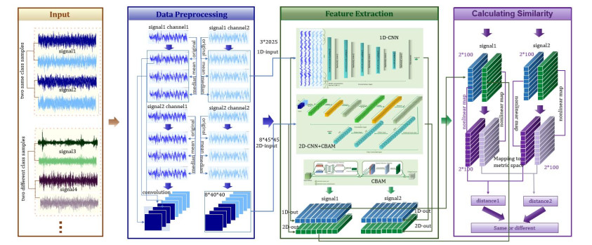
Bearings are critical components of industrial equipment and have a significant impact on the safety of industrial physical systems. Their failure may lead to equipment shutdown and accidents, posing a significant risk to production safety. However, it is difficult to obtain a large amount of bearing fault data in practice, which makes the problem of small sample size a major challenge for bearing fault detection. In addition, some methods may overlook important features in bearing vibration signals, leading to insufficient detection capabilities. To address the challenges in bearing fault detection, this paper proposed a few sample learning methods based on the multidimensional convolution and attention mechanism. First, a multichannel preprocessing method was designed to more effectively utilize the information in the bearing vibration signal. Second, by extracting multidimensional features and enhancing the attention to important features through multidimensional convolution operations and attention mechanisms, the feature extraction ability of the network was improved. Furthermore, nonlinear mapping of feature vectors into the metric space to calculate distance can better measure the similarity between samples, thereby improving the accuracy of bearing fault detection and providing important guarantees for the safe operation of industrial systems. Extensive experiments have shown that the proposed method has good fault detection performance under small sample conditions, which is beneficial for reducing machine downtime and economic losses.

References

[1]	N. W. Nirwan, H. B. Ramani, Condition monitoring and fault detection in roller bearing used in rolling mill by acoustic emission and vibration analysis, Mater. Today Proc., 51 (2022), 344–354. https://doi.org/10.1016/j.matpr.2021.05.447 doi: 10.1016/j.matpr.2021.05.447
[2]	S. Rajabi, M. S. Azari, S. Santini, F. Flammini, Fault diagnosis in industrial rotating equipment based on permutation entropy, signal processing and multi-output neuro-fuzzy classifier, Expert Syst. Appl., 206 (2022), 117754. https://doi.org/10.1016/j.eswa.2022.117754 doi: 10.1016/j.eswa.2022.117754
[3]	E. A. Burda, G. V. Zusman, I. S. Kudryavtseva, A. P. Naumenko, An overview of vibration analysis techniques for the fault diagnostics of rolling bearings in machinery, Shock Vib., 2022 (2022). https://doi.org/10.1155/2022/6136231 doi: 10.1155/2022/6136231
[4]	J. Gu, Y. Peng, H. Lu, X. Chang, G. Chen, A novel fault diagnosis method of rotating machinery via VMD, CWT and improved CNN, Measurement, 200 (2022), 111635. https://doi.org/10.1016/j.measurement.2022.111635 doi: 10.1016/j.measurement.2022.111635
[5]	J. Pacheco-Chérrez, J. A. Fortoul-Díaz, F. Cortés-Santacruz, L. M. Aloso-Valerdi, D. I. Ibarra-Zarate, Bearing fault detection with vibration and acoustic signals: Comparison among different machine leaning classification methods, Eng. Fail. Anal., 139 (2022), 106515. https://doi.org/10.1016/j.engfailanal.2022.106515 doi: 10.1016/j.engfailanal.2022.106515
[6]	K. Berg-Sørensen, H. Flyvbjerg, Power spectrum analysis for optical tweezers, Rev. Sci. Instrum., 75 (2004), 594–612. https://doi.org/10.1063/1.1645654 doi: 10.1063/1.1645654
[7]	R. B. Randall, A history of cepstrum analysis and its application to mechanical problems, Mech. Syst. Signal Process., 97 (2017), 3–19. https://doi.org/10.1016/j.ymssp.2016.12.026 doi: 10.1016/j.ymssp.2016.12.026
[8]	A. R. Al-Obaidi, H. J. Towsyfyan, An experimental study on vibration signatures for detecting incipient cavitation in centrifugal pumps based on envelope spectrum analysis, J. Appl. Fluid Mech., 12 (2019), 2057–2067. https://doi.org/10.29252/JAFM.12.06.29901 doi: 10.29252/JAFM.12.06.29901
[9]	N. Peifeng, Z. Jun, Z. Gang, Study on application of wavelet transform technique to turbine generator fault diagnosis, Chin. J. Sci. Instrum., 28 (2007), 188. https://doi.org/10.19650/j.cnki.cjsi.2007.01.039 doi: 10.19650/j.cnki.cjsi.2007.01.039
[10]	P. Konar, P. Chattopadhyay, Bearing fault detection of induction motor using wavelet and support vector machines (SVMs), Appl. Soft Comput., 11 (2011), 4203–4211. https://doi.org/10.1016/j.asoc.2011.03.014 doi: 10.1016/j.asoc.2011.03.014
[11]	N. E. Huang, Z. Shen, S. R. Long, M. C. Wu, H. H. Shih, Q. Zheng, et al., The empirical mode decomposition and the Hilbert spectrum for nonlinear and non-stationary time series analysis, Proc. R. Soc. London, 454 (1998), 903–995. https://doi.org/10.1098/rspa.1998.0193 doi: 10.1098/rspa.1998.0193
[12]	C. Song, S. Liu, G. Han, P. Zeng, H. Yu, Q. Zheng, Edge-intelligence-based condition monitoring of beam pumping units under heavy noise in industrial internet of things for industry 4.0, IEEE Int. Things J., 10 (2023), 3037–3046. https://doi.org/10.1109/JIOT.2022.3141382 doi: 10.1109/JIOT.2022.3141382
[13]	S. Liu, C. Song, T. Wu, P. Zeng, A lightweight fault diagnosis method of beam pumping units based on dynamic warping matching and parallel deep network, IEEE Trans. Syst., Man, Cybern., 54 (2023), 1622–1632. https://doi.org/10.1109/TSMC.2023.3328731 doi: 10.1109/TSMC.2023.3328731
[14]	Q. Cui, Z. Li, J. Yang, B. Liang, Rolling bearing fault prognosis using recurrent neural network, in 2017 29th Chinese Control And Decision Conference (CCDC), (2017), 1196–1201. https://doi.org/10.1109/CCDC.2017.7978700
[15]	L. Yu, J. Qu, F. Gao, Y. Tian, A novel hierarchical algorithm for bearing fault diagnosis based on stacked LSTM, Shock Vib., 2019 (2019). https://doi.org/10.1155/2019/2756284 doi: 10.1155/2019/2756284
[16]	C. Song, P. Zeng, Z. Wang, T. Li, L. Qiao, L. Shen, Image forgery detection based on motion blur estimated using convolutional neural network, IEEE Sens. J., 19 (2019), 11601–11611. https://doi.org/10.1109/JSEN.2019.2928480 doi: 10.1109/JSEN.2019.2928480
[17]	M. Ye, X. Yan, D. Jiang, L. Xiang, N. Chen, MIFDELN: A multi-sensor information fusion deep ensemble learning network for diagnosing bearing faults in noisy scenarios, Knowl.-Based Syst., 284 (2024), 111294. https://doi.org/10.1016/j.knosys.2023.111294 doi: 10.1016/j.knosys.2023.111294
[18]	X. Yan, W. J. Yan, Y. Xu, K. V. Yuen, Machinery multi-sensor fault diagnosis based on adaptive multivariate feature mode decomposition and multi-attention fusion residual convolutional neural network, Mech. Syst. Signal Process., 202, (2023), 110664. https://doi.org/10.1016/j.ymssp.2023.11066 doi: 10.1016/j.ymssp.2023.11066
[19]	X. Yan, D. She, Y. Xu, Deep order-wavelet convolutional variational autoencoder for fault identification of rolling bearing under fluctuating speed conditions, Expert Syst. Appl., 216 (2023), 119479. https://doi.org/10.1016/j.eswa.2022.119479 doi: 10.1016/j.eswa.2022.119479
[20]	H. Liu, H. Zhao, J. Wang, S. Yuan, W. Feng, LSTM-GAN-AE: A promising approach for fault diagnosis in machine health monitoring, IEEE Trans. Instrum. Meas., 71 (2021), 1–13. https://doi.org/10.1109/TIM.2021.3135328 doi: 10.1109/TIM.2021.3135328
[21]	J. Yang, J. Liu, J. Xie, C. Wang, T. Ding, Conditional GAN and 2-D CNN for bearing fault diagnosis with small samples, IEEE Trans. Instrum. Meas., 70 (2021), 1–12. https://doi.org/10.1109/TIM.2021.3119135 doi: 10.1109/TIM.2021.3119135
[22]	G. Yang, C. Song, Z. Yang, S. Cui, Bubble detection in photoresist with small samples based on GAN augmentations and modified YOLO, Eng. Appl. Artif. Intell., 123 (2023), 106224. https://doi.org/10.1016/j.engappai.2023.106224 doi: 10.1016/j.engappai.2023.106224
[23]	C. Song, W. Xu, Z. Wang, S. Yu, Z. Ju, Analysis on the impact of data augmentation on target recognition for UAV-based transmission line inspection, Complexity, 2020 (2020). https://doi.org/10.1155/2020/3107450 doi: 10.1155/2020/3107450
[24]	O. Bohdal, Y. Tian, Y. Zong, R. Chavhan, D. Li, H. Gouk, et al., Meta omnium: A benchmark for general-purpose learning-to-learn, in 2023 IEEE/CVF Conference on Computer Vision and Pattern Recognition (CVPR), (2023), 7693–7703. https://doi.org/10.1109/CVPR52729.2023.00743
[25]	K. Song, J. Han, G. Cheng, J. Lu, F. Nie, Adaptive neighborhood metric learning, IEEE Trans. Pattern Anal. Mach. Intell., 44 (2022), 4591-4604. https://doi.org/10.1109/TPAMI.2021.3073587 doi: 10.1109/TPAMI.2021.3073587
[26]	Z. Wu, H. Jiang, K. Zhao, X. Li, An adaptive deep transfer learning method for bearing fault diagnosis, Measurement, 151 (2020), 107227. https://doi.org/10.1016/j.measurement.2019.107227 doi: 10.1016/j.measurement.2019.107227
[27]	J. Zhu, N. Chen, C. Shen, A new deep transfer learning method for bearing fault diagnosis under different working conditions, IEEE Sens. J., 20 (2019), 8394–8402. https://doi.org/10.1109/jsen.2019.2936932 doi: 10.1109/jsen.2019.2936932
[28]	B. Yang, Y. Lei, F. Jia, S. Xing, An intelligent fault diagnosis approach based on transfer learning from laboratory bearings to locomotive bearings, Mech. Syst. Signal Process., 122 (2019), 692–706. https://doi.org/10.1016/j.ymssp.2018.12.051 doi: 10.1016/j.ymssp.2018.12.051
[29]	X. Li, Y. Hu, M. Li, J. Zheng, Fault diagnostics between different type of components: A transfer learning approach, Appl. Soft Comput., 86, (2020), 105950. https://doi.org/10.1016/j.asoc.2019.105950 Get rights and content
[30]	Y. F. Li, M. Zuo, K. Feng, Y. J. Chen, Detection of bearing faults using a novel adaptive morphological update lifting wavelet, Chin. J. Mech. Eng., 30 (2017), 1305–1313. https://doi.org/10.1007/s10033-017-0186-1 doi: 10.1007/s10033-017-0186-1
[31]	Q. Fu, B. Jing, P. He, S. Si, Y. Wang, Fault feature selection and diagnosis of rolling bearings based on EEMD and optimized Elman_AdaBoost algorithm, IEEE Sens. J., 18 (2018), 5024–5034. https://doi.org/10.1109/JSEN.2018.2830109 doi: 10.1109/JSEN.2018.2830109
[32]	J. Zheng, S. Huang, H. Pan, J. Tong, C. Wang, Q. Liu, Adaptive power spectrum Fourier decomposition method with application in fault diagnosis for rolling bearing, Measurement, 183 (2021), 109837. https://doi.org/10.1016/j.measurement.2021.109837 doi: 10.1016/j.measurement.2021.109837
[33]	K. Feng, Q. Ni, M. Beer, H. Du, C. Li, A novel similarity-based status characterization methodology for gear surface wear propagation monitoring, Tribol. Int., 174 (2022), 107765.
[34]	K. Feng, J. C. Ji, Y. Zhang, Q. Ni, Z. Liu, M. Beer, Digital twin-driven intelligent assessment of gear surface degradation, Mech. Syst. Signal Process., 186 (2023), 109896. https://doi.org/10.1016/j.ymssp.2022.109896 doi: 10.1016/j.ymssp.2022.109896
[35]	Q. Ni, J. C. Ji, B. Halkon, K. Feng, A. K. Nandi, Physics-informed pesidual network (PIResNet) for rolling element bearing fault diagnostics, Mech. Syst. Signal Process., 200 (2023), 110544. https://doi.org/10.1016/j.ymssp.2023.110544 doi: 10.1016/j.ymssp.2023.110544
[36]	D. Peng, Z. Liu, H. Wang, Y. Qin, L. Jia, A novel deeper one-dimensional CNN with residual learning for fault diagnosis of wheelset bearings in high-speed trains, IEEE Access, 7 (2018), 10278–10293. https://doi.org/10.1109/ACCESS.2018.2888842 doi: 10.1109/ACCESS.2018.2888842
[37]	X. Peng, B. Zhang, D. Gao, Research on fault diagnosis method of rolling bearing based on 2DCNN, in 2020 Chinese Control And Decision Conference (CCDC), (2020), 693–697. https://doi.org/10.26914/c.cnkihy.2020.033919
[38]	D. Wang, Q. Guo, Y. Song, S. Gao, Y. Li, Application of multiscale learning neural network based on CNN in bearing fault diagnosis, J. Signal Process. Syst., 91 (2019), 1205–1217. https://doi.org/10.1007/s11265-019-01461-w doi: 10.1007/s11265-019-01461-w
[39]	A. Khorram, M. Khalooei, M. Rezghi, End-to-end CNN+ LSTM deep learning approach for bearing fault diagnosis, Appl. Intell., 51 (2021), 736–751. https://doi.org/10.1007/s10489-020-01859-1 doi: 10.1007/s10489-020-01859-1
[40]	W. Zhang, G. Peng, C. Li, Y. Chen, Z. Zhang, A new deep learning model for fault diagnosis with good anti-noise and domain adaptation ability on raw vibration signals, Sensors, 17, (2017), 425. https://doi.org/10.3390/s17020425 doi: 10.3390/s17020425
[41]	A. Zhang, S. Li, Y. Cui, W. Yang, R. Dong, J. Hu, Limited data rolling bearing fault diagnosis with few-shot learning, IEEE Access, 7 (2019), 110895–110904. https://doi.org/10.1109/ACCESS.2019.2934233 doi: 10.1109/ACCESS.2019.2934233

Reader Comments

Your name:*

Email:*
© 2024 the Author(s), licensee AIMS Press. This is an open access article distributed under the terms of the Creative Commons Attribution License (http://creativecommons.org/licenses/by/4.0)