Lagrange tracking-based long-term drift trajectory prediction method for Autonomous Underwater Vehicle

Shuwen Zheng; Mingjun Zhang; Jing Zhang; Jitao Li; Shuwen Zheng; Mingjun Zhang; Jing Zhang; Jitao Li

doi:10.3934/mbe.2023932

Mathematical Biosciences and Engineering

2023, Volume 20, Issue 12: 21075-21097. doi: 10.3934/mbe.2023932

Previous Article Next Article

Research article

Lagrange tracking-based long-term drift trajectory prediction method for Autonomous Underwater Vehicle

1.
College of Mechanical and Electrical Engineering, Harbin Engineering University, Harbin 150001, China
2.
School of Information Science and Engineering, University of Jinan, Jinan 250022, China

Academic Editor: Hamid Reza Karim

Received: 27 August 2023 Revised: 20 November 2023 Accepted: 21 November 2023 Published: 27 November 2023

Autonomous Underwater Vehicle (AUV) works autonomously in complex marine environments. After a severe accident, an AUV will lose its power and rely on its small buoyancy to ascend at a slow speed. If the reserved buoyancy is insufficient, when reaching the thermocline, the buoyancy will rapidly decrease to zero. Consequently, the AUV will experience prolonged lateral drift within the thermocline. This study focuses on developing a prediction method for the drift trajectory of an AUV after a long-term power loss accident. The aim is to forecast the potential resurfacing location, providing technical support for surface search and salvage operations of the disabled AUV. To the best of our knowledge, currently, there is no mature and effective method for predicting long-term AUV underwater drift trajectories. In response to this issue, based on real AUV catastrophes, this paper studies the prediction of long-term AUV underwater drift trajectories in the cases of power loss. We propose a three-dimensional trajectory prediction method based on the Lagrange tracking approach. This method takes the AUV's longitudinal velocity, the time taken to reach different depths, and ocean current data at various depths into account. The reason for the AUV's failure to ascend to sea surface lies that the remaining buoyancy is too small to overcome the thermocline. As a result, AUV drifts long time within the thermocline. To address this issue, a method for estimating thermocline currents is proposed, which can be used to predict the lateral drift trajectory of the AUV within the thermocline. Simulation is conducted to compare the results obtained by the proposed method and that in a real accident. The results demonstrate that the proposed approach exhibits small directional and positional errors. This validates the effectiveness of the proposed method.
- AUV,
- underwater drift,
- lagrange tracking method,
- track prediction
Citation: Shuwen Zheng, Mingjun Zhang, Jing Zhang, Jitao Li. Lagrange tracking-based long-term drift trajectory prediction method for Autonomous Underwater Vehicle[J]. Mathematical Biosciences and Engineering, 2023, 20(12): 21075-21097. doi: 10.3934/mbe.2023932

Related Papers:

Abstract

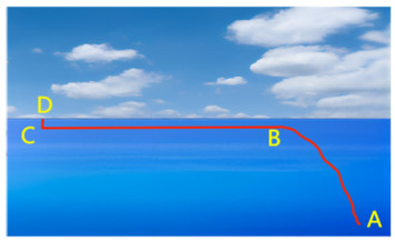
Autonomous Underwater Vehicle (AUV) works autonomously in complex marine environments. After a severe accident, an AUV will lose its power and rely on its small buoyancy to ascend at a slow speed. If the reserved buoyancy is insufficient, when reaching the thermocline, the buoyancy will rapidly decrease to zero. Consequently, the AUV will experience prolonged lateral drift within the thermocline. This study focuses on developing a prediction method for the drift trajectory of an AUV after a long-term power loss accident. The aim is to forecast the potential resurfacing location, providing technical support for surface search and salvage operations of the disabled AUV. To the best of our knowledge, currently, there is no mature and effective method for predicting long-term AUV underwater drift trajectories. In response to this issue, based on real AUV catastrophes, this paper studies the prediction of long-term AUV underwater drift trajectories in the cases of power loss. We propose a three-dimensional trajectory prediction method based on the Lagrange tracking approach. This method takes the AUV's longitudinal velocity, the time taken to reach different depths, and ocean current data at various depths into account. The reason for the AUV's failure to ascend to sea surface lies that the remaining buoyancy is too small to overcome the thermocline. As a result, AUV drifts long time within the thermocline. To address this issue, a method for estimating thermocline currents is proposed, which can be used to predict the lateral drift trajectory of the AUV within the thermocline. Simulation is conducted to compare the results obtained by the proposed method and that in a real accident. The results demonstrate that the proposed approach exhibits small directional and positional errors. This validates the effectiveness of the proposed method.

References

[1]	X. Xiang, C. Yu, Q. Zhang, On intelligent risk analysis and critical decision of underwater robotic vehicle, Ocean Eng., 140 (2017), 453–465. https://doi.org/10.1016/j.oceaneng.2017.06.020 doi: 10.1016/j.oceaneng.2017.06.020
[2]	W. Wawrzyński, M. Zieja, M. Żokowski, N. Sigiel, Optimization of Autonomous Underwater Vehicle mission planning process, Bull. Pol. Acad. Sci. Tech. Sci., 70 (2022), e140371. https://doi.org/10.24425/bpasts.2022.140371 doi: 10.24425/bpasts.2022.140371
[3]	X. Chen, N. Bose, M. Brito, F. Khan, B. Thanyamanta, T. Zou, A review of risk analysis research for the operations of Autonomous Underwater Vehicles, Reliab. Eng. Syst. Saf., 216 (2021), 108011. https://doi.org/10.1016/j.ress.2021.108011 doi: 10.1016/j.ress.2021.108011
[4]	S. Xia, X. Zhou, H. Shi, S. Li, C. Xu, A fault diagnosis method based on attention mechanism with application in Qianlong-2 Autonomous Underwater Vehicle, Ocean Eng., 233 (2021), 109049. https://doi.org/10.1016/j.oceaneng.2021.109049 doi: 10.1016/j.oceaneng.2021.109049
[5]	D. Chaos, D. Moreno-Salinas, J. Aranda, Fault-tolerant control for AUVs using a single thruster, IEEE Access, 10 (2022), 22123–22139. https://doi.org/10.1109/access.2022.3152190 doi: 10.1109/ACCESS.2022.3152190
[6]	Y. Yu, J. Zhang, T. Zhang, AUV drift track prediction method based on a modified neural network, Appl. Sci., 12 (2022), 12169. https://doi.org/10.3390/app122312169 doi: 10.3390/app122312169
[7]	S. Meng, W. Lu, Y. Li, H. Wang, L. Jiang, A study on the leeway drift characteristic of a typical fishing vessel common in the Northern South China Sea, Appl. Ocean Res., 109 (2021), 102498. https://doi.org/10.1016/j.apor.2020.102498 doi: 10.1016/j.apor.2020.102498
[8]	H. Tu, L. Mu, K. Xia, X. Wang, K. Zhu, Determining the drift characteristics of open lifeboats based on large-scale drift experiments, Front. Mar. Sci., 9 (2022), 1017042. https://doi.org/10.3389/fmars.2022.1017042 doi: 10.3389/fmars.2022.1017042
[9]	J. R. Frost, L. D. Stone, Review of search theory: Advances and applications to search and rescue decision support, TRB Annu. Meet., 2001.
[10]	National SAR Manual, National Search and Rescue Manual, EXHIBIT/P-00112, 1998. Available from: http://www.oshsi.nl.ca/userfiles/files/p00112.pdf.
[11]	L. P. Perera, P. Oliveira, C. Guedes Soares, Maritime traffic monitoring based on vessel detection, tracking, state estimation, and trajectory prediction, IEEE Trans. Intell. Transp. Syst., 13 (2012), 1188–1200. https://doi.org/10.1109/tits.2012.2187282 doi: 10.1109/TITS.2012.2187282
[12]	J. Zhang, Â. P. Teixeira, C. Guedes Soares, X. Yan, Probabilistic modelling of the drifting trajectory of an object under the effect of wind and current for maritime search and rescue, Ocean Eng., 129 (2017), 253–264. https://doi.org/10.1016/j.oceaneng.2016.11.002 doi: 10.1016/j.oceaneng.2016.11.002
[13]	P. Miron, F. J. Beron-Vera, M. J. Olascoaga, P. Koltai, Markov-chain-inspired search for MH370, Chaos: Interdiscip. J. Nonlinear Sci., 29 (2019), 041105. https://doi.org/10.1063/1.5092132 doi: 10.1063/1.5092132
[14]	M. Zhao, J. Zhang, M. H. Rashid, Predicting the drift position of ships using deep learning, in the 2nd International Conference on Computing and Data Science, Association for Computing Machinery, (2021), 1–5. https://doi.org/10.1145/3448734.3450922
[15]	A. A. Pereira, J. Binney, G. A. Hollinger, G. S. Sukhatme, Risk-aware path planning for Autonomous Underwater Vehicles using Predictive ocean models, J. Field Rob., 30 (2013), 741–762. https://doi.org/10.1002/rob.21472 doi: 10.1002/rob.21472
[16]	D. N. Subramani, Q. J. Wei, P. F. J. Lermusiaux, Stochastic time-optimal path-planning in uncertain, strong, and dynamic flows, Comput. Methods Appl. Mech. Eng., 333 (2018), 218–237. https://doi.org/10.1016/j.cma.2018.01.004 doi: 10.1016/j.cma.2018.01.004
[17]	Z. Wu, H. R. Karimi, C. Dang, An approximation algorithm for graph partitioning via deterministic annealing neural network, Neural Networks, 117 (2019), 191–200. https://doi.org/10.1016/j.neunet.2019.05.010 doi: 10.1016/j.neunet.2019.05.010
[18]	Z. Wu, Q. Gao, B. Jiang, H. R. Karimi, Solving the production transportation problem via a deterministic annealing neural network method, Appl. Math. Comput., 411 (2021), 126518. https://doi.org/10.1016/j.amc.2021.126518 doi: 10.1016/j.amc.2021.126518
[19]	D. Tong, B. Ma, Q. Chen, Y. Wei, P. Shi, Finite-time synchronization and energy consumption prediction for multilayer fractional-order networks, IEEE Trans. Circuits Syst. Ⅱ Express Briefs, 70 (2023), 2176–2180. https://doi.org/10.1109/TCSII.2022.3233420 doi: 10.1109/TCSII.2022.3233420
[20]	G. Yang, D. Tong, Q. Chen, W. Zhou, Fixed-time synchronization and energy consumption for kuramoto-oscillator networks with multilayer distributed control, IEEE Trans. Circuits Syst. Ⅱ Express Briefs, 70 (2022), 1555–1559. https://doi.org/10.1109/TCSII.2022.3221477 doi: 10.1109/TCSII.2022.3221477
[21]	C. Xu, D. Tong, Q. Chen, W. Zhou, P. Shi, Exponential stability of Markovian jump systems via adaptive sliding mode control, IEEE Trans. Syst. Man Cybern.: Syst., 51 (2019), 954–964. https://doi.org/10.1109/TSMC.2018.2884565 doi: 10.1109/TSMC.2018.2884565
[22]	K. Zhu, L. Mu, H. Tu, Exploration of the wind-induced drift characteristics of typical Chinese offshore fishing vessels, Appl. Ocean Res., 92 (2019), 101916. https://doi.org/10.1016/j.apor.2019.101916 doi: 10.1016/j.apor.2019.101916
[23]	H. Yasukawa, N. Hirata, Y. Nakayama, A. Matsuda, Drifting of a dead ship in wind, Ship Technol. Res., 70 (2023), 26–45. https://doi.org/10.1080/09377255.2021.1954835 doi: 10.1080/09377255.2021.1954835
[24]	H. W. Tu, X. D. Wang, L. Mu, J. L. Sun, A study on the drift prediction method of wrecked fishing vessels at sea, in OCEANS 2021: San Diego–Porto, IEEE, (2021), 1–6. https://doi.org/10.23919/OCEANS44145.2021.9705751
[25]	D. Sumangala, A. Joshi, H. Warrior, Modelling freshwater plume in the Bay of Bengal with artificial neural networks, Curr. Sci., 123 (2022), 73–80. https://doi.org/10.18520/cs/v123/i1/73-80 doi: 10.18520/cs/v123/i1/73-80
[26]	L. Ren, Z. Hu, M. Hartnett, Short-term forecasting of coastal surface currents using high frequency radar data and artificial neural networks, Remote Sens., 10 (2018), 850. https://doi.org/10.3390/rs10060850 doi: 10.3390/rs10060850
[27]	H. Kalinić, H. Mihanović, S. Cosoli, M. Tudor, I. Vilibić, Predicting ocean surface currents using numerical weather prediction model and Kohonen neural network: A northern Adriatic study, Neural Comput. Appl., 28 (2017), 611–620. https://doi.org/10.1007/s00521-016-2395-4 doi: 10.1007/s00521-016-2395-4
[28]	H. Guan, X. Dong, C. Xue, Z. Luo, H. Yang, T. Wu, Optimization of POM based on parallel supercomputing grid cloud platform, in 2019 Seventh International Conference on Advanced Cloud and Big Data (CBD), IEEE, (2019), 49–54. https://doi.org/10.1109/cbd.2019.00019
[29]	A. K. Das, A. Sharma, S. Joseph, A. Srivastava, D. R. Pattanaik, Comparative performance of HWRF model coupled with POM and HYCOM for tropical cyclones over North Indian Ocean, MAUSAM, 72 (2021), 147–166. https://doi.org/10.54302/mausam.v72i1.127 doi: 10.54302/mausam.v72i1.127
[30]	C. D. Dong, T. H. H. Nguyen, T. H. Hou, C. C. Tsai, Integrated numerical model for the simulation of the T.S. Taipei oil spill, J. Mar. Sci. Technol., 27 (2019), 7. https://doi.org/10.6119/JMST.201908_27(4).0007 doi: 10.6119/JMST.201908_27(4).0007
[31]	J. Xu, J. Y. Bao, C. Y. Zhan, X. H. Zhou, Tide model CST1 of China and its application for the water level reducer of bathymetric data, Mar. Geod., 40 (2017), 74–86. https://doi.org/10.1080/01490419.2017.1308896 doi: 10.1080/01490419.2017.1308896
[32]	H. Xu, Tracking lagrange trajectories in position–velocity space, Meas. Sci. Technol., 19 (2008), 075105. https://doi.org/10.1088/0957-0233/19/7/075105 doi: 10.1088/0957-0233/19/7/075105
[33]	T. Heus, G. van Dijk, H. J. J. Jonker, H. E. A. Van den Akker, Mixing in shallow cumulus clouds studied by lagrange particle tracking, J. Atmos. Sci., 65 (2008), 2581–2597. https://doi.org/10.1175/2008jas2572.1 doi: 10.1175/2008JAS2572.1
[34]	N. B. Engdahl, R. M. Maxwell, Quantifying changes in age distributions and the hydrologic balance of a high-mountain watershed from climate induced variations in recharge, J. Hydrol., 522 (2015), 152–162. https://doi.org/10.1016/j.jhydrol.2014.12.032 doi: 10.1016/j.jhydrol.2014.12.032
[35]	M. Jing, F. Heße, R. Kumar, O. Kolditz, T. Kalbacher, S. Attinger, Influence of input and parameter uncertainty on the prediction of catchment-scale groundwater travel time distributions, Hydrol. Earth Syst. Sci., 23 (2019), 171–190. https://doi.org/10.5194/hess-23-171-2019 doi: 10.5194/hess-23-171-2019
[36]	Y. H. Zhu, S. Q. Peng, 40 years of marine data products in the south china sea (1980–2019) (1/10 degree) (hourly) (netcdf), the Key Special Project for Introduced Talents Team of Southern Marine Science and Engineering Guangdong Laboratory (Guangzhou) (GML2019ZD0303), 2019. Available from: http://data.scsio.ac.cn/metaDatadetail/1480813599763386368.
[37]	NOOA Physical Sciences Laboratory (PSL), NCEP/NCAR Reanalysis. Available from: https://psl.noaa.gov/.
[38]	W. Ekman, Eddy-viscosity and skin-friction in the dynamics of winds and ocean-currents, in Memoirs of the Royal Meteorological Society, Stanford, (1928), 161–172.
[39]	N. P. Fofonoff, Physical properties of seawater: A new salinity scale and equation of state for seawater, J. Geophys. Res., 90 (1985), 3332–3342. https://doi.org/10.1029/JC090iC02p03332 doi: 10.1029/JC090iC02p03332
[40]	Y. Jiang, Y. Li, Y. Su, J. Cao, Y. Li, Y. Wang, et al., Statics variation analysis due to spatially moving of a full ocean depth Autonomous Underwater Vehicle, Int. J. Nav. Archit. Ocean Eng., 11 (2019), 448–461. https://doi.org/10.1016/j.ijnaoe.2018.08.002 doi: 10.1016/j.ijnaoe.2018.08.002
[41]	K. Zhang, New gravity acceleration formula research (in Chinese), Prog. Geophys., 26 (2011), 824–828. https://doi.org/10.3969/j.issn.1004-2903.2011.03.006 doi: 10.3969/j.issn.1004-2903.2011.03.006
[42]	Y. K. Wang, Simulation research on the full-ocean-depth AUV diving and floating motion (in Chinese), Harbin Eng. Univ., 2020. https://doi.org/10.27060/d.cnki.ghbcu.2019.000077 doi: 10.27060/d.cnki.ghbcu.2019.000077
[43]	A. Chen, J. Ye, Research on four-layer back propagation neural network for the computation of ship resistance, in 2009 International Conference on Mechatronics and Automation, IEEE, (2009), 2537–2541. https://doi.org/10.1109/icma.2009.5245975
[44]	X. Chen, C. Wei, G. Zhou, H. Wu, Z. Wang, S. A. Biancardo, Automatic identification system (AIS) data supported ship trajectory prediction and analysis via a deep learning model, J. Mar. Sci. Eng., 10 (2022), 1314. https://doi.org/10.3390/jmse10091314 doi: 10.3390/jmse10091314

Reader Comments

Your name:*

Email:*
© 2023 the Author(s), licensee AIMS Press. This is an open access article distributed under the terms of the Creative Commons Attribution License (http://creativecommons.org/licenses/by/4.0)