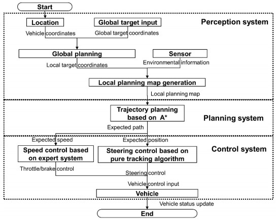
Trajectory planning is one of the key technologies for autonomous driving. A* algorithm is a classical trajectory planning algorithm that has good results in the field of robot path planning. However, there are still some practical problems to be solved when the algorithm is applied to vehicles, such as the algorithm fails to consider the vehicle contours, the planned path is not smooth, and it lacks speed planning. In order to solve these problems, this paper proposes a path processing method and a path tracking method for the A* algorithm. First, the method of configuring safe redundancy space is given considering the vehicle contour, then, the path is generated based on A* algorithm and smoothed using Bessel curve, and the speed is planned based on the curvature of the path. The trajectory tracking algorithm in this paper is based on an expert system and pure tracking theory. In terms of speed tracking, an expert system for the acceleration characteristics of the vehicle is constructed and used as a priori information for speed control, and good results are obtained. In terms of path tracking, the required steering wheel angle is calculated based on pure tracking theory, and the influence factor of speed on steering is obtained from test data, based on which the steering wheel angle is corrected and the accuracy of path tracking is improved. In addition, this paper proposes a target point selection method for the pure tracking algorithm to improve the stability of vehicle directional control. Finally, a simulation analysis of the proposed method is performed. The results show that the method can improve the applicability of the A* algorithm in automated vehicle planning.
Citation: Xiaoyong Xiong, Haitao Min, Yuanbin Yu, Pengyu Wang. Application improvement of A* algorithm in intelligent vehicle trajectory planning[J]. Mathematical Biosciences and Engineering, 2021, 18(1): 1-21. doi: 10.3934/mbe.2021001
Trajectory planning is one of the key technologies for autonomous driving. A* algorithm is a classical trajectory planning algorithm that has good results in the field of robot path planning. However, there are still some practical problems to be solved when the algorithm is applied to vehicles, such as the algorithm fails to consider the vehicle contours, the planned path is not smooth, and it lacks speed planning. In order to solve these problems, this paper proposes a path processing method and a path tracking method for the A* algorithm. First, the method of configuring safe redundancy space is given considering the vehicle contour, then, the path is generated based on A* algorithm and smoothed using Bessel curve, and the speed is planned based on the curvature of the path. The trajectory tracking algorithm in this paper is based on an expert system and pure tracking theory. In terms of speed tracking, an expert system for the acceleration characteristics of the vehicle is constructed and used as a priori information for speed control, and good results are obtained. In terms of path tracking, the required steering wheel angle is calculated based on pure tracking theory, and the influence factor of speed on steering is obtained from test data, based on which the steering wheel angle is corrected and the accuracy of path tracking is improved. In addition, this paper proposes a target point selection method for the pure tracking algorithm to improve the stability of vehicle directional control. Finally, a simulation analysis of the proposed method is performed. The results show that the method can improve the applicability of the A* algorithm in automated vehicle planning.

| [1] | Z. Wang, W. Du, J. Wang, J. Zhou, X. Han, Z. Zhang, et al., Research and application of improved adaptive MOMEDA fault diagnosis method, Measurement., 140 (2019), 63-75. |
| [2] |
B. Gao, Q. Yang, Z. Peng, W. Xie, H. Jin, S. Meng, A direct random sampling method for the Fourier amplitude sensitivity test of nonuniformly distributed uncertainty inputs and its application in C/C nozzles, Aerosp. Sci. Technol., 100 (2020), 105830-105837. doi: 10.1016/j.ast.2020.105830

|
| [3] | H. Chen, H. Chen, Q. Liu, Three dimensional formation path planning of multiple UAVs based on improved artificial potential field method, J. Syst. Simul., 1 (2019), 1-7. |
| [4] |
Y. Li, R. Wang, Y. Liu, M. Xu, Satellite range scheduling with the priority constraint: An improved genetic algorithm using a station ID encoding method, Chin. J. Aeronaut., 28 (2015), 789-803. doi: 10.1016/j.cja.2015.04.012
|
| [5] |
H. Wang, W. Mao, L. Eriksson, A Three-Dimensional Dijkstra's algorithm for multi-objective ship voyage optimization, Ocean Eng., 186 (2019), 106131-106143. doi: 10.1016/j.oceaneng.2019.106131
|
| [6] | B. Fu, L. Chen, Y. Zhou, D. Zheng, Z. Wei, J. Dai, et al., An improved A* algorithm for the industrial robot path planning with high success rate and short length, Rob. Auton. Syst., 106 (2018), 26-37. |
| [7] | F. Zhang, W. Bai, Y. Qiao, B. Xing, P. Zhou, UAV indoor path planning based on improved D*algorithm, CAAI Trans. Intell. Syst., 14 (2019), 662-669. |
| [8] |
G. D. Goez, R. A. Velasquez, J. S. Botero, UAV route planning optimization using PSO implemented on microcontrollers, IEEE Lat. Am. Trans., 14 (2016), 1705-1710. doi: 10.1109/TLA.2016.7483504
|
| [9] | H. Min, X. Xiong, P. Wang, Y. Yu, Autonomous driving path planning algorithm based on improved A* algorithm in unstructured environment, Proc. Inst. Mech. Eng., Part D., 2020 (2020), 0954407020959741. |
| [10] | Y. Zhang, Y. Zhao, T. Wei, Improved A* algorithm for obstacle avoidance path planning strategy of the blind, Aero Weaponry., 3 (2017), 86-92. |
| [11] | F. Islam, V. Narayanan, M. Likhachev, A*-Connect: Bounded suboptimal bidirectional heuristic search, 2016 IEEE International Conference on Robotics and Automation (ICRA), 2016. Available from: https://ieeexplore.ieee.org/abstract/document/7487437. |
| [12] | Z. Zhang, T. Long, Z. Wang, G. Xu, Y. Cao, UAV dynamic path planning using anytime repairing sparse A* algorithm and targets motion estimation, 2018 IEEE CSAA Guidance, Navigation and Control Conference (CGNCC), 2018. Available from: https://ieeexplore.ieee.org/abstract/document/9019099. |
| [13] |
K. Mi, J. Zheng, Y. Wang, J. Hu, A multi-heuristic A* algorithm based on stagnation detection for path planning of manipulators in cluttered environments, IEEE Access, 7 (2019), 135870-135881. doi: 10.1109/ACCESS.2019.2941537
|
| [14] | F. Islam, V. Narayanan, M. Likhachev, Dynamic multi-heuristic A*, 2015 IEEE International Conference on Robotics and Automation (ICRA), 2015. Available from: https://ieeexplore.ieee.org/abstract/document/7139515. |
| [15] | Q. Wan, C. Gu, S. Sun, M. Chen, H. Huang, X. Jia, Lifelong multi-agent path finding in a dynamic environment, 2018 15th International Conference on Control, Automation, Robotics and Vision (ICARCV), 2018. Available from: https://ieeexplore.ieee.org/abstract/document/8581181. |
| [16] |
F. A. Raheem, U. I. Hameed, Heuristic D* algorithm based on particle swarm optimization for path planning of two-link robot arm in dynamic environment, Al-Khwarizmi Eng. J., 15 (2019), 108-123. doi: 10.22153/kej.2019.01.004
|
| [17] | S. Oh, H. W. Leong, Strict Theta*: shorter motion path planning using taut paths, Proceedings of the Twenty-Sixth International Conference on International Conference on Automated Planning and Scheduling, 2016. Available from: https://dl.acm.org/doi/abs/10.5555/3038594.3038626. |
| [18] | B. Cui, M. Wang, Y. Duan, Path planning for a* algorithm based on searching 24 neighborhoods, J. Shenyang Univ. Technol., 40 (2018), 180-184. |
| [19] | F. Christ, A. Wischnewski, A. Heilmeier, B. Lohmann, Time-optimal trajectory planning for a race car considering variable tyre-road friction coefficients. Veh. Syst. Dyn., 2019 (2019), 1-25. |
| [20] |
Y. Zhang, B. Gao, L. Guo, H. Guo, M. Cui, A novel trajectory planning method for automated vehicles under parameter decision framework, IEEE Access, 7 (2019), 88264-88274. doi: 10.1109/ACCESS.2019.2925417
|
| [21] | Z. Wang, J. Zha, J. Wang, Flatness-based model predictive control for autonomous vehicle trajectory tracking, 2019 IEEE Intelligent Transportation Systems Conference (ITSC), 2019. Available from: https://ieeexplore.ieee.org/abstract/document/8917260. |
| [22] | H. Wang, X. Chen, Y. Chen, B. Li, Z. Miao, Trajectory tracking and speed control of cleaning vehicle based on improved pure pursuit algorithm*, 2019 Chinese Control Conference (CCC), 2019. Available from: https://ieeexplore.ieee.org/abstract/document/8865255. |
| [23] | A. V. Le, V. Prabakaran, V. Sivanantham, R. E. Mohan, Modified a-star algorithm for efficient coverage path planning in tetris inspired self-reconfigurable robot with integrated laser sensor, Sensors, 18 (2018), 2585-2612. |
| [24] |
S. K. Renny, N. Uchiyama, S. Sano, Real-time smooth trajectory generation for nonholonomic mobile robots using Bezier curves, Rob. Comput. Integr. Manuf., 41 (2016), 31-42. doi: 10.1016/j.rcim.2016.02.002
|
| [25] | J. Duan, C. Yang, H. Shi, Path tracking based on pure pursuit algorithm for intelligent vehicles, J. Beijing Univ. Technol., 42 (2016), 1301-1306. |


Figures(21) / Tables(2)

Xiaoyong Xiong, Haitao Min, Yuanbin Yu, Pengyu Wang. Application improvement of A* algorithm in intelligent vehicle trajectory planning[J]. Mathematical Biosciences and Engineering, 2021, 18(1): 1-21. doi: 10.3934/mbe.2021001


 DownLoad: