Wave interference network with a wave function for traffic sign recognition

Qiang Weng; Dewang Chen; Yuandong Chen; Wendi Zhao; Lin Jiao; Qiang Weng; Dewang Chen; Yuandong Chen; Wendi Zhao; Lin Jiao

doi:10.3934/mbe.2023851

Mathematical Biosciences and Engineering

2023, Volume 20, Issue 11: 19254-19269. doi: 10.3934/mbe.2023851

Previous Article Next Article

Research article Special Issues

Wave interference network with a wave function for traffic sign recognition

School of Transportation, Fujian University of Technology, Fuzhou 350118, China

Academic Editor: Shangce Gao

Received: 04 August 2023 Revised: 19 September 2023 Accepted: 26 September 2023 Published: 16 October 2023

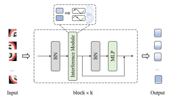
In this paper, we successfully combine convolution with a wave function to build an effective and efficient classifier for traffic signs, named the wave interference network (WiNet). In the WiNet, the feature map extracted by the convolutional filters is refined into many entities from an input image. Each entity is represented as a wave. We utilize Euler's formula to unfold the wave function. Based on the wave-like information representation, the model modulates the relationship between the entities and the fixed weights of convolution adaptively. Experiment results on the Chinese Traffic Sign Recognition Database (CTSRD) and the German Traffic Sign Recognition Benchmark (GTSRB) demonstrate that the performance of the presented model is better than some other models, such as ResMLP, ResNet50, PVT and ViT in the following aspects: 1) WiNet obtains the best accuracy rate with 99.80% on the CTSRD and recognizes all images exactly on the GTSRB; 2) WiNet gains better robustness on the dataset with different noises compared with other models; 3) WiNet has a good generalization on different datasets.

Keywords:

Citation: Qiang Weng, Dewang Chen, Yuandong Chen, Wendi Zhao, Lin Jiao. Wave interference network with a wave function for traffic sign recognition[J]. Mathematical Biosciences and Engineering, 2023, 20(11): 19254-19269. doi: 10.3934/mbe.2023851

Related Papers:

[1]	Giuseppe Maria Coclite, Lorenzo di Ruvo . A singular limit problem for conservation laws related to the Kawahara-Korteweg-de Vries equation. Networks and Heterogeneous Media, 2016, 11(2): 281-300. doi: 10.3934/nhm.2016.11.281
[2]	Hyeontae Jo, Hwijae Son, Hyung Ju Hwang, Eun Heui Kim . Deep neural network approach to forward-inverse problems. Networks and Heterogeneous Media, 2020, 15(2): 247-259. doi: 10.3934/nhm.2020011
[3]	Anya Désilles, Hélène Frankowska . Explicit construction of solutions to the Burgers equation with discontinuous initial-boundary conditions. Networks and Heterogeneous Media, 2013, 8(3): 727-744. doi: 10.3934/nhm.2013.8.727
[4]	Tong Yan . The numerical solutions for the nonhomogeneous Burgers' equation with the generalized Hopf-Cole transformation. Networks and Heterogeneous Media, 2023, 18(1): 359-379. doi: 10.3934/nhm.2023014
[5]	Jinyi Sun, Weining Wang, Dandan Zhao . Global existence of 3D rotating magnetohydrodynamic equations arising from Earth's fluid core. Networks and Heterogeneous Media, 2025, 20(1): 35-51. doi: 10.3934/nhm.2025003
[6]	Guillermo Reyes, Juan-Luis Vázquez . The Cauchy problem for the inhomogeneous porous medium equation. Networks and Heterogeneous Media, 2006, 1(2): 337-351. doi: 10.3934/nhm.2006.1.337
[7]	Caihong Gu, Yanbin Tang . Global solution to the Cauchy problem of fractional drift diffusion system with power-law nonlinearity. Networks and Heterogeneous Media, 2023, 18(1): 109-139. doi: 10.3934/nhm.2023005
[8]	Bendong Lou . Self-similar solutions in a sector for a quasilinear parabolic equation. Networks and Heterogeneous Media, 2012, 7(4): 857-879. doi: 10.3934/nhm.2012.7.857
[9]	Yannick Holle, Michael Herty, Michael Westdickenberg . New coupling conditions for isentropic flow on networks. Networks and Heterogeneous Media, 2020, 15(4): 605-631. doi: 10.3934/nhm.2020016
[10]	Flavia Smarrazzo, Alberto Tesei . Entropy solutions of forward-backward parabolic equations with Devonshire free energy. Networks and Heterogeneous Media, 2012, 7(4): 941-966. doi: 10.3934/nhm.2012.7.941

Abstract

1. Introduction

The equation:

$\begin{equation} \begin{cases} \partial_t u + \partial_x f(u)-\beta^2 \partial_{x}^2 u+\delta \partial_{x}^3 u+\kappa u +\gamma^2\vert u\vert u = 0, &\quad 0 < t < T, \quad x\in \mathbb{R},\\ u(0,x) = u_0(x), &\quad x\in \mathbb{R}, \end{cases} \end{equation}$

(1.1)

was originally derived in ^[14,17] with $f(u) = au^2$ focusing on microbubbles coated by viscoelastic shells. These structures are crucial in ultrasound diagnosis using contrast agents, and the dynamics of individual coated bubbles are explored, taking into account nonlinear competition and dissipation factors such as dispersion, thermal effects, and drag force.

The coefficients $\beta^2$ , $\delta$ , $\kappa$ , and $\gamma^2$ are related to the dissipation, the dispersion, the thermal conduction dissipation, and to the drag force, repsctively.

If $\kappa = \gamma = 0$ , we obtain the Kudryashov-Sinelshchikov ^[18] Korteweg-de Vries-Burgers ^[3,20] equation

$\begin{equation} \partial_t u +a \partial_x u^2-\beta^2 \partial_{x}^2 u+\delta \partial_{x}^3 u = 0, \end{equation}$

(1.2)

that models pressure waves in liquids with gas bubbles, taking into account heat transfer and viscosity. The mathematical results on Eq (1.2) are the following:

● analysis of exact solutions in ^[13],

● existence of the traveling waves in ^[2],

● well-posedness and asymptotic behavior in ^[7,11].

If $\beta = 0$ , we derive the Korteweg-de Vries equation:

$\begin{equation} \partial_t u +a \partial_x u^2+\delta \partial_{x}^3 u = 0, \end{equation}$

(1.3)

which describes surface waves of small amplitude and long wavelength in shallow water. Here, $u(t, x)$ represents the wave height above a flat bottom, $x$ corresponds to the distance in the propagation direction, and $t$ denotes the elapsed time. In ^{[4,6,10,12,15,16]}, the completele integrability of Eq (1.3) and the existence of solitary wave solutions are proved.

Through the manuscript, we will assume

● on the coefficients

$\begin{equation} \beta,\,\delta,\,\kappa,\,\gamma\in \mathbb{R}, \quad \beta,\,\delta,\,\gamma\ne0; \end{equation}$

(1.4)

● on the flux $f$ , one of the following conditions:

$\begin{align} &f(u) = a u^2+bu^3, \end{align}$

(1.5)

$\begin{align} &f\in C^1( \mathbb{R}), \quad \vert f'(u)\vert\le C_0\left(1+\vert u\vert\right), \quad u\in \mathbb{R}, \end{align}$

(1.6)

for some positive constant $C_0$ ;

● on the initial value

$\begin{equation} u_0\in H^1( \mathbb{R}). \end{equation}$

(1.7)

The main result of this paper is the following theorem.

Theorem 1.1. Assume Eqs (1.5)–(1.7). For fixed $T > 0$ , there exists a unique distributional solution $u$ of Eq (1.1), such that

$\begin{equation} \begin{split} u \in&\, L^{\infty}(0,T;H^1( \mathbb{R}))\cap L^4(0,\,T;W^{1,\,4}( \mathbb{R}))\cap L^6(0,\,T;W^{1,\,6}( \mathbb{R}))\\ \partial_{x}^2 u\in&\, L^2((0,\,T)\times \mathbb{R}). \end{split} \end{equation}$

(1.8)

Moreover, if $u_1$ and $u_2$ are solutions to Eq (1.1) corresponding to the initial conditions $u_{1, 0}$ and $u_{2, 0}$ , respectively, it holds that:

$\begin{equation} \left\| {u_1(t,\cdot)-u_2(t,\cdot)} \right\|_{L^2( \mathbb{R})}\le e^{C(T)t}\left\| {u_{1,0}-u_{2,0}} \right\|_{L^2( \mathbb{R})}, \end{equation}$

(1.9)

for some suitable $C(T) > 0$ , and every, $0\le t\le T$ .

Observe that Theorem 1.1 gives the well-posedness of (1.1), without conditions on the constants. Moreover, the proof of Theorem 1.1 is based on the Aubin-Lions Lemma ^[5,21]. The analysis of Eq (1.1) is more delicate than the one of Eq (1.2) due to the presence of the nonlinear sources and the very general assumptions on the coefficients.

The structure of the paper is outlined as follows. Section 2 is dedicated to establishing several a priori estimates for a vanishing viscosity approximation of Eq (1.1). These estimates are crucial for proving our main result, which is presented in Section 3.

2. Vanishing viscosity approximation

To establish existence, we utilize a vanishing viscosity approximation of equation (1.1), as discussed in ^[19]. Let $0 < \varepsilon < 1$ be a small parameter, and denote by $u_\varepsilon\in C^\infty([0, T)\times \mathbb{R})$ the unique classical solution to the following problem ^[1,9]:

$\begin{equation} \begin{cases} \partial_t u_\varepsilon + \partial_x f( u_\varepsilon)-\beta^2 \partial_{x}^2 u_\varepsilon+\delta \partial_{x}^3 u_\varepsilon+\kappa u\\ \qquad\quad +\gamma^2\vert u\vert u = - \varepsilon \partial_{x}^4 u_\varepsilon, &\quad 0 < t < T, \quad x\in \mathbb{R},\\ u_{ \varepsilon}(0,x) = u_{ \varepsilon,\,0}(x), &\quad x\in \mathbb{R}, \end{cases} \end{equation}$

(2.1)

where $u_{ \varepsilon, \, 0}$ is a $C^{\infty}$ approximation of $u_0$ , such that

$\begin{equation} \left\| {u_{ \varepsilon,\,0}} \right\|_{H^1( \mathbb{R})}\le \left\| {u_0} \right\|_{H^1( \mathbb{R})}. \end{equation}$

(2.2)

Let us prove some a priori estimates on $u_\varepsilon$ , denoting with $C_0$ constants which depend only on the initial data, and with $C(T)$ the constants which depend also on $T$ .

We begin by proving the following lemma:

Lemma 2.1. Let $T > 0$ be fixed. There exists a constant $C(T) > 0$ , which does not depend on $\varepsilon$ , such that

$\begin{equation} \begin{split} \left\| { u_\varepsilon(t,\cdot)} \right\|^2_{L^2( \mathbb{R})}&+2\gamma^2e^{\vert\kappa\vert t}\displaystyle {\int}_{0}^{t}\!\!\displaystyle {\int}_{ \mathbb{R}}e^{-\vert\kappa\vert s} u_\varepsilon^2\vert u_\varepsilon\vert dsdx\\ &+2\beta^2e^{\vert\kappa\vert t}\displaystyle {\int}_{0}^{t}e^{-\vert\kappa\vert s}\left\| { \partial_x u_\varepsilon(s,\cdot)} \right\|^2_{L^2( \mathbb{R})} ds\\ &+2 \varepsilon e^{\vert\kappa\vert t}\displaystyle {\int}_{0}^{t}e^{-\vert\kappa\vert s}\left\| { \partial_{x}^2 u_\varepsilon(s,\cdot)} \right\|^2_{L^2(R)}\le C(T), \end{split} \end{equation}$

(2.3)

for every $0\le t\le T$ .

Proof. For $0\le t\le T$ . Multiplying equations (2.1) by $2 u_\varepsilon$ , and integrating over $\mathbb{R}$ yields

$\begin{align*} \frac{d}{dt}&\left\| { u_\varepsilon(t,\cdot)} \right\|^2_{L^2( \mathbb{R})} = 2\displaystyle {\int}_{ \mathbb{R}} u_\varepsilon \partial_t u_\varepsilon dx\\ = &\underbrace{-2\displaystyle {\int}_{ \mathbb{R}} u_\varepsilon f'( u_\varepsilon) \partial_x u_\varepsilon dx}_{ = 0}+2\beta^2\displaystyle {\int}_{ \mathbb{R}} u_\varepsilon \partial_{x}^2 u_\varepsilon dx-2\delta\displaystyle {\int}_{ \mathbb{R}} u_\varepsilon \partial_{x}^3 u_\varepsilon dx \\ &-\kappa\left\| { u_\varepsilon(t,\cdot)} \right\|^2_{L^2( \mathbb{R})}-2\gamma^2\displaystyle {\int}_{ \mathbb{R}}\vert u_\varepsilon\vert u_\varepsilon^2 dx-2 \varepsilon\displaystyle {\int}_{ \mathbb{R}} u_\varepsilon \partial_{x}^4 u_\varepsilon dx \\ = &-2\beta^2\left\| { \partial_x u_\varepsilon(t,\cdot)} \right\|^2_{L^2( \mathbb{R})}+2\delta\displaystyle {\int}_{ \mathbb{R}} \partial_x u_\varepsilon \partial_{x}^2 u_\varepsilon dx\\ &-\kappa\left\| { u_\varepsilon(t,\cdot)} \right\|^2_{L^2( \mathbb{R})}-2\gamma^2\displaystyle {\int}_{ \mathbb{R}}\vert u_\varepsilon\vert u_\varepsilon^2 dx+2 \varepsilon\displaystyle {\int}_{ \mathbb{R}} \partial_x u_\varepsilon \partial_{x}^3 u_\varepsilon dx\\ = &-2\beta^2\left\| { \partial_x u_\varepsilon(t,\cdot)} \right\|^2_{L^2( \mathbb{R})}-\kappa\left\| { u_\varepsilon(t,\cdot)} \right\|^2_{L^2( \mathbb{R})}\\ &-2\gamma^2\displaystyle {\int}_{ \mathbb{R}}\vert u_\varepsilon\vert u_\varepsilon^2 dx-2 \varepsilon\left\| { \partial_{x}^2 u_\varepsilon(t,\cdot)} \right\|^2_{L^2( \mathbb{R})}. \end{align*}$

Thus, it follows that

$\begin{align*} \frac{d}{dt}\left\| { u_\varepsilon(t,\cdot)} \right\|^2_{L^2( \mathbb{R})}+&2\beta^2\left\| { \partial_x u_\varepsilon(t,\cdot)} \right\|^2_{L^2( \mathbb{R})}\\ &+2\gamma^2\displaystyle {\int}_{ \mathbb{R}}\vert u_\varepsilon\vert u_\varepsilon^2 dx+2 \varepsilon\left\| { \partial_{x}^2 u_\varepsilon(t,\cdot)} \right\|^2_{L^2( \mathbb{R})}\\ = &\kappa\left\| { u_\varepsilon(t,\cdot)} \right\|^2_{L^2( \mathbb{R})}\le \vert\kappa\vert \left\| { u_\varepsilon(t,\cdot)} \right\|^2_{L^2( \mathbb{R})}. \end{align*}$

Therefore, applying the Gronwall's lemma and using Eq (2.2), we obtain

$\begin{align*} \left\| { u_\varepsilon(t,\cdot)} \right\|^2_{L^2( \mathbb{R})}&+2\beta^2 e^{\vert\kappa\vert t}\displaystyle {\int}_{0}^{t}e^{-\vert\kappa\vert s}\left\| { \partial_x u_\varepsilon(s,\cdot)} \right\|^2_{L^2( \mathbb{R})}ds\\ &+ 2\gamma^2e^{\vert\kappa\vert t}\displaystyle {\int}_{0}^t\!\!\displaystyle {\int}_{ \mathbb{R}}e^{-\vert\kappa\vert t}\vert u_\varepsilon\vert u_\varepsilon^2 dsdx+2 \varepsilon\left\| { \partial_{x}^2 u_\varepsilon(t,\cdot)} \right\|^2_{L^2( \mathbb{R})}\\ &+2 \varepsilon e^{\vert\kappa\vert t}\displaystyle {\int}_{0}^{t}e^{-\vert\kappa\vert s} \left\| { \partial_{x}^2 u_\varepsilon(s,\cdot)} \right\|^2_{L^2( \mathbb{R})}ds\\ \le& C_0e^{\vert\kappa\vert t}\le C(T), \end{align*}$

which gives Eq (2.3). □

Lemma 2.2. Fix $T > 0$ and assume (1.5). There exists a constant $C(T) > 0$ , independent of $\varepsilon$ , such that

$\begin{align} \left\| { u_\varepsilon} \right\|_{L^{\infty}((0,T)\times \mathbb{R})}&\le C(T), \end{align}$

(2.4)

$\begin{align} \left\| { \partial_x u_\varepsilon(t,\cdot)} \right\|^2_{L^2( \mathbb{R})}+\beta^2\displaystyle {\int}_{0}^{t}\left\| { \partial_{x}^2 u_\varepsilon(s,\cdot)} \right\|^2_{L^2( \mathbb{R})}ds& \end{align}$

(2.5)

$\begin{align} +2 \varepsilon\displaystyle {\int}_{0}^{t}\left\| { \partial_{x}^3 u_\varepsilon(s,\cdot)} \right\|^2_{L^2( \mathbb{R})}ds&\le C(T),\\ \displaystyle {\int}_{0}^{t}\left\| { \partial_x u_\varepsilon(s,\cdot)} \right\|^4_{L^4( \mathbb{R})} ds&\le C(T), \end{align}$

(2.6)

holds for every $0\le t\le T$ .

Proof. Let $0\le t\le T$ . Consider $A, \, B$ as two real constants, which will be specified later. Thanks to Eq (1.5), multiplying Eq (2.1) by

$\begin{equation*} -2 \partial_{x}^2 u_\varepsilon+A u_\varepsilon^2+B u_\varepsilon^3, \end{equation*}$

we have that

$\begin{align} &\left(-2 \partial_{x}^2 u_\varepsilon+A u_\varepsilon^2+B u_\varepsilon^3\right) \partial_t u_\varepsilon+ 2a\left(-2 \partial_{x}^2 u_\varepsilon+A u_\varepsilon^2+B u_\varepsilon^3\right) u_\varepsilon \partial_x u_\varepsilon\\ &\qquad\quad+3b\left(-2 \partial_{x}^2 u_\varepsilon+A u_\varepsilon^2+B u_\varepsilon^3\right) u_\varepsilon^2 \partial_x u_\varepsilon-\beta^2\left(-2 \partial_{x}^2 u_\varepsilon+A u_\varepsilon^2+B u_\varepsilon^3\right) \partial_{x}^2 u_\varepsilon \\ &\qquad\quad+\delta\left(-2 \partial_{x}^2 u_\varepsilon+A u_\varepsilon^2+B u_\varepsilon^3\right) \partial_{x}^3 u_\varepsilon+\kappa\left(-2 \partial_{x}^2 u_\varepsilon+A u_\varepsilon^2+B u_\varepsilon^3\right) u_\varepsilon\\ &\qquad\quad+\gamma^2\left(-2 \partial_{x}^2 u_\varepsilon+A u_\varepsilon^2+B u_\varepsilon^3\right)\vert u_\varepsilon\vert u_\varepsilon = - \varepsilon\left(-2 \partial_{x}^2 u_\varepsilon+A u_\varepsilon^2+B u_\varepsilon^3\right) \partial_{x}^4 u_\varepsilon. \end{align}$

(2.7)

Observe that

$\begin{align*} &\displaystyle {\int}_{ \mathbb{R}}\left(-2 \partial_{x}^2 u_\varepsilon+A u_\varepsilon^2+B u_\varepsilon^3\right) \partial_t u_\varepsilon dx\\ &\qquad = \frac{d}{dt}\left(\left\| { \partial_x u_\varepsilon(t,\cdot)} \right\|^2_{L^2( \mathbb{R})}+\frac{A}{3}\displaystyle {\int}_{ \mathbb{R}} u_\varepsilon^3dx +\frac{B}{4}\displaystyle {\int}_{ \mathbb{R}} u_\varepsilon^4 dx\right),\\ &2a\displaystyle {\int}_{ \mathbb{R}}\left(-2 \partial_{x}^2 u_\varepsilon+A u_\varepsilon^2+B u_\varepsilon^3\right) u_\varepsilon \partial_x u_\varepsilon dx = -4a\displaystyle {\int}_{ \mathbb{R}} u_\varepsilon \partial_x u_\varepsilon \partial_{x}^2 u_\varepsilon dx,\\ &3b\displaystyle {\int}_{ \mathbb{R}}\left(-2 \partial_{x}^2 u_\varepsilon+A u_\varepsilon^2+B u_\varepsilon^3\right) u_\varepsilon^2 \partial_x u_\varepsilon dx = -6b\displaystyle {\int}_{ \mathbb{R}} u_\varepsilon^2 \partial_x u_\varepsilon \partial_{x}^2 u_\varepsilon dx,\\ &{-\beta^2\displaystyle {\int}_{ \mathbb{R}}\left(-2 \partial_{x}^2 u_\varepsilon+A u_\varepsilon^2+B u_\varepsilon^3\right) \partial_{x}^2 u_\varepsilon dx}\\ &\qquad = 2\beta^2\left\| { \partial_{x}^2 u_\varepsilon(t,\cdot)} \right\|^2_{L^2( \mathbb{R})}+2A\beta^2\displaystyle {\int}_{ \mathbb{R}} u_\varepsilon( \partial_x u_\varepsilon)^2 dx +3B\beta^2\displaystyle {\int}_{ \mathbb{R}} u_\varepsilon^2( \partial_x u_\varepsilon)^2dx, \\ &\delta\displaystyle {\int}_{ \mathbb{R}}\left(-2 \partial_{x}^2 u_\varepsilon+A u_\varepsilon^2+B u_\varepsilon^3\right) \partial_{x}^3 u_\varepsilon dx = -2A\delta\displaystyle {\int}_{ \mathbb{R}} u_\varepsilon \partial_x u_\varepsilon \partial_{x}^2 u_\varepsilon dx -3B\delta\displaystyle {\int}_{ \mathbb{R}} u_\varepsilon^2 \partial_x u_\varepsilon \partial_{x}^2 u_\varepsilon dx, \\ &\kappa\displaystyle {\int}_{ \mathbb{R}}\left(-2 \partial_{x}^2 u_\varepsilon+A u_\varepsilon^2+B u_\varepsilon^3\right) u_\varepsilon dx\\ &\qquad = {2\kappa\left\| { \partial_x u_\varepsilon(t,\cdot)} \right\|^2_{L^2( \mathbb{R})}+{A\kappa}\displaystyle {\int}_{ \mathbb{R}} u_\varepsilon^3 dx +{B\kappa}\displaystyle {\int}_{ \mathbb{R}} u_\varepsilon^4 dx,}\\ &\gamma^2\displaystyle {\int}_{ \mathbb{R}}\left(-2 \partial_{x}^2 u_\varepsilon+A u_\varepsilon^2+B u_\varepsilon^3\right)\vert u_\varepsilon\vert u_\varepsilon dx\\ &\qquad = -2\gamma^2\displaystyle {\int}_{ \mathbb{R}}\vert u_\varepsilon\vert u_\varepsilon \partial_{x}^2 u_\varepsilon dx +A\gamma^2\displaystyle {\int}_{ \mathbb{R}}\vert u\vert u_\varepsilon^3dx +B\gamma^2\displaystyle {\int}_{ \mathbb{R}}\vert u_\varepsilon\vert u^4 dx,\\ &- \varepsilon\displaystyle {\int}_{ \mathbb{R}}\left(-2 \partial_{x}^2 u_\varepsilon+A u_\varepsilon^2+B u_\varepsilon^3\right) \partial_{x}^4 u_\varepsilon dx\\ &\qquad = -2 \varepsilon\left\| { \partial_{x}^3 u_\varepsilon(t,\cdot)} \right\|^2_{L^2( \mathbb{R})}+2A \varepsilon\displaystyle {\int}_{ \mathbb{R}} u_\varepsilon \partial_x u_\varepsilon{ \partial_{x}^3 u_\varepsilon} dx+3B \varepsilon\displaystyle {\int}_{ \mathbb{R}} u_\varepsilon^2 \partial_x u_\varepsilon \partial_{x}^3 u_\varepsilon dx\\ &\qquad = -2 \varepsilon\left\| { \partial_{x}^3 u_\varepsilon(t,\cdot)} \right\|^2_{L^2( \mathbb{R})}-A \varepsilon\displaystyle {\int}_{ \mathbb{R}}( \partial_x u_\varepsilon)^3 dx -6B \varepsilon\displaystyle {\int}_{ \mathbb{R}} u_\varepsilon( \partial_x u_\varepsilon)^2 \partial_{x}^2 u_\varepsilon dx\\ &\qquad\quad -3B \varepsilon\left\| { u_\varepsilon(t,\cdot) \partial_{x}^2 u_\varepsilon(t,\cdot)} \right\|^2_{L^2( \mathbb{R})}\\ &\qquad = -2 \varepsilon\left\| { \partial_{x}^3 u_\varepsilon(t,\cdot)} \right\|^2_{L^2( \mathbb{R})}-A \varepsilon\displaystyle {\int}_{ \mathbb{R}}( \partial_x u_\varepsilon)^3 dx +2B \varepsilon\displaystyle {\int}_{ \mathbb{R}}( \partial_x u_\varepsilon)^4dx\\ &\qquad\quad -3B \varepsilon\left\| { u_\varepsilon(t,\cdot) \partial_{x}^2 u_\varepsilon(t,\cdot)} \right\|^2_{L^2( \mathbb{R})}. \end{align*}$

Therefore, an integration on $\mathbb{R}$ gives

$\begin{align*} &\frac{d}{dt}\left(\left\| { \partial_x u_\varepsilon(t,\cdot)} \right\|^2_{L^2( \mathbb{R})}+\frac{A}{3}\displaystyle {\int}_{ \mathbb{R}} u_\varepsilon^3dx +\frac{B}{4}\displaystyle {\int}_{ \mathbb{R}} u_\varepsilon^4 dx\right)\\ &\qquad\quad +\beta^2\left\| { \partial_{x}^2 u_\varepsilon(t,\cdot)} \right\|^2_{L^2( \mathbb{R})}+2 \varepsilon\left\| { \partial_{x}^3 u_\varepsilon(t,\cdot)} \right\|^2_{L^2( \mathbb{R})}\\ &\qquad = -\left(4a+A\delta\right)\displaystyle {\int}_{ \mathbb{R}} u_\varepsilon \partial_x u_\varepsilon \partial_{x}^2 u_\varepsilon dx -3\left(2b+B\delta\right)\displaystyle {\int}_{ \mathbb{R}} u_\varepsilon^2 \partial_x u_\varepsilon \partial_{x}^2 u_\varepsilon dx\\ &\qquad\quad -2A\beta^2\displaystyle {\int}_{ \mathbb{R}} u_\varepsilon( \partial_x u_\varepsilon)^2 dx -3B\beta^2\displaystyle {\int}_{ \mathbb{R}} u_\varepsilon^2( \partial_x u_\varepsilon)^2dx\\ &\qquad\quad -\kappa\left\| { \partial_x u_\varepsilon(t,\cdot)} \right\|^2_{L^2( \mathbb{R})}-\frac{A\kappa}{3}\displaystyle {\int}_{ \mathbb{R}} u_\varepsilon^3 dx -\frac{B\kappa}{4}\displaystyle {\int}_{ \mathbb{R}} u_\varepsilon^4 dx\\ &\qquad\quad +2\gamma^2\displaystyle {\int}_{ \mathbb{R}}\vert u_\varepsilon\vert u_\varepsilon \partial_{x}^2 u_\varepsilon dx {-A\gamma^2\displaystyle {\int}_{ \mathbb{R}}\vert u_\varepsilon\vert u_\varepsilon^3dx-B\gamma^2\displaystyle {\int}_{ \mathbb{R}}\vert u_\varepsilon\vert u_\varepsilon^4 dx}\\ &\qquad\quad -A \varepsilon\displaystyle {\int}_{ \mathbb{R}}( \partial_x u_\varepsilon)^3 dx +2B \varepsilon\displaystyle {\int}_{ \mathbb{R}}( \partial_x u_\varepsilon)^4dx-3B \varepsilon\left\| { u_\varepsilon(t,\cdot) \partial_{x}^2 u_\varepsilon(t,\cdot)} \right\|^2_{L^2( \mathbb{R})}. \end{align*}$

Taking

$\begin{equation*} \left(A,\,B\right) = \left(-\frac{4a}{\delta},\,-\frac{2b}{\delta}\right), \end{equation*}$

we get

$\begin{align} &\frac{d}{dt}\left(\left\| { \partial_x u_\varepsilon(t,\cdot)} \right\|^2_{L^2( \mathbb{R})}-\frac{4a}{3\delta}\displaystyle {\int}_{ \mathbb{R}} u_\varepsilon^3dx -\frac{b}{\delta}\displaystyle {\int}_{ \mathbb{R}} u_\varepsilon^4 dx\right)\\ &\qquad\quad +2\beta^2\left\| { \partial_{x}^2 u_\varepsilon(t,\cdot)} \right\|^2_{L^2( \mathbb{R})}+2 \varepsilon\left\| { \partial_{x}^3 u_\varepsilon(t,\cdot)} \right\|^2_{L^2( \mathbb{R})}\\ &\qquad = \frac{8a\beta^2}{\delta}\displaystyle {\int}_{ \mathbb{R}} u_\varepsilon( \partial_x u_\varepsilon)^2 dx +\frac{6b\beta^2}{\delta}\displaystyle {\int}_{ \mathbb{R}} u_\varepsilon^2( \partial_x u_\varepsilon)^2dx\\ &\qquad\quad -\kappa\left\| { \partial_x u_\varepsilon(t,\cdot)} \right\|^2_{L^2( \mathbb{R})}+\frac{4a\kappa}{3\delta}\displaystyle {\int}_{ \mathbb{R}} u_\varepsilon^3 dx +\frac{b\kappa}{2}\displaystyle {\int}_{ \mathbb{R}} u_\varepsilon^4 dx\\ &\qquad\quad +2\gamma^2\displaystyle {\int}_{ \mathbb{R}}\vert u_\varepsilon\vert u_\varepsilon \partial_{x}^2 u_\varepsilon dx {+\frac{4a\gamma^2}{\delta}\displaystyle {\int}_{ \mathbb{R}}\vert u_\varepsilon\vert u_\varepsilon^3dx +\frac{2b\gamma^2}{\delta}\displaystyle {\int}_{ \mathbb{R}}\vert u_\varepsilon\vert u_\varepsilon^4 dx} \\ &\qquad\quad +\frac{4a \varepsilon}{\delta}\displaystyle {\int}_{ \mathbb{R}}( \partial_x u_\varepsilon)^3 dx-\frac{4b \varepsilon}{\delta}\displaystyle {\int}_{ \mathbb{R}}( \partial_x u_\varepsilon)^4dx+\frac{6b \varepsilon}{\delta}\left\| { u_\varepsilon(t,\cdot) \partial_{x}^2 u_\varepsilon(t,\cdot)} \right\|^2_{L^2( \mathbb{R})}. \end{align}$

(2.8)

Since $0 < \varepsilon < 1$ , due to the Young inequality and (2.3),

$\begin{align*} &\frac{8a\beta^2}{\delta}\displaystyle {\int}_{ \mathbb{R}}\vert u_\varepsilon\vert( \partial_x u_\varepsilon)^2 dx\\ &\qquad\le 4\displaystyle {\int}_{ \mathbb{R}} u_\varepsilon^2( \partial_x u_\varepsilon)^2 dx +\frac{4a^2\beta^4}{\delta^2}\left\| { \partial_x u_\varepsilon(t,\cdot)} \right\|^2_{L^2( \mathbb{R})}\\ &\qquad\le 4\left\| { u_\varepsilon} \right\|^2_{L^{\infty}((0,T)\times \mathbb{R})}\left\| { \partial_x u_\varepsilon(t,\cdot)} \right\|^2_{L^2( \mathbb{R})}+\frac{4a^2\beta^4}{\delta^2}\left\| { \partial_x u_\varepsilon(t,\cdot)} \right\|^2_{L^2( \mathbb{R})}\\ &\qquad\le C_0\left(1+\left\| { u_\varepsilon} \right\|^2_{L^{\infty}((0,T)\times \mathbb{R})}\right)\left\| { \partial_x u_\varepsilon(t,\cdot)} \right\|^2_{L^2( \mathbb{R})},\\ &\left\vert\frac{6b\beta^2}{\delta}\right\vert\displaystyle {\int}_{ \mathbb{R}} u_\varepsilon^2( \partial_x u_\varepsilon)^2dx\le \left\vert\frac{6b\beta^2}{\delta}\right\vert\left\| { u_\varepsilon} \right\|^2_{L^{\infty}((0,T)\times \mathbb{R})}\left\| { \partial_x u_\varepsilon(t,\cdot)} \right\|^2_{L^2( \mathbb{R})},\\ &\vert\frac{4a\kappa}{3\delta}\vert\displaystyle {\int}_{ \mathbb{R}}\vert u_\varepsilon\vert^3 dx\le \left\vert\frac{4a\kappa}{3\delta}\right\vert\left\| { u_\varepsilon} \right\|_{L^{\infty}((0,T)\times \mathbb{R})}\left\| { u_\varepsilon(t,\cdot)} \right\|^2_{L^2( \mathbb{R})}\\ &\qquad\le C(T)\left\| { u_\varepsilon} \right\|_{L^{\infty}((0,T)\times \mathbb{R})},\\ &\left\vert\frac{b\kappa}{2}\right\vert\displaystyle {\int}_{ \mathbb{R}} u_\varepsilon^4 dx\le \left\vert\frac{b\kappa}{2}\right\vert\left\| { u_\varepsilon} \right\|^2_{L^{\infty}((0,T)\times \mathbb{R})}\left\| { u_\varepsilon(t,\cdot)} \right\|^2_{L^2( \mathbb{R})}\\ &\qquad\le C(T)\left\| { u_\varepsilon} \right\|^2_{L^{\infty}((0,T)\times \mathbb{R})}, \\ &2\gamma^2\displaystyle {\int}_{ \mathbb{R}}\vert u_\varepsilon\vert u_\varepsilon \partial_{x}^2 u_\varepsilon dx{\le}2\displaystyle {\int}_{ \mathbb{R}}\left\vert\frac{\gamma^2\vert u_\varepsilon\vert u_\varepsilon}{\beta}\right\vert\left\vert\beta \partial_{x}^2 u_\varepsilon\right\vert dx\\ &\qquad\le\frac{\gamma^4}{\beta^2}\displaystyle {\int}_{ \mathbb{R}}{ u_\varepsilon}^4dx +\beta^2\left\| { \partial_{x}^2 u_\varepsilon(t,\cdot)} \right\|^2_{L^2( \mathbb{R})}\\ &\qquad \le\frac{\gamma^4}{\beta^2}\left\| { u_\varepsilon} \right\|^2_{L^{\infty}((0.T)\times \mathbb{R})}\left\| { u_\varepsilon(t,\cdot)} \right\|^2_{L^2( \mathbb{R})} +\beta^2\left\| { \partial_{x}^2 u_\varepsilon(t,\cdot)} \right\|^2_{L^2( \mathbb{R})}\\ &\qquad\le C(T)\left\| { u_\varepsilon} \right\|^2_{L^{\infty}((0,T)\times \mathbb{R})}+\beta^2\left\| { \partial_{x}^2 u_\varepsilon(t,\cdot)} \right\|^2_{L^2( \mathbb{R})},\\ &\left\vert\frac{4a\gamma^2}{\delta}\right\vert\displaystyle {\int}_{ \mathbb{R}}\vert { u_\varepsilon}\vert \vert u_\varepsilon\vert^3dx = \left\vert\frac{4a\gamma^2}{\delta}\right\vert\displaystyle {\int}_{ \mathbb{R}} u_\varepsilon^4 dx\\ &\qquad\le \left\vert\frac{4a\gamma^2}{\delta}\right\vert\left\| { u_\varepsilon} \right\|^2_{L^{\infty}((0,T)\times \mathbb{R})}\left\| { u_\varepsilon(t,\cdot)} \right\|^2_{L^2( \mathbb{R})} \le C(T)\left\| { u_\varepsilon} \right\|^2_{L^{\infty}((0,T)\times \mathbb{R})}, \\ &\left\vert\frac{2b\gamma^2}{\delta}\right\vert\displaystyle {\int}_{ \mathbb{R}}\vert u_\varepsilon\vert { u_\varepsilon}^4 dx\le \left\vert\frac{2b\gamma^2}{\delta}\right\vert\left\| { u_\varepsilon} \right\|^3_{L^{\infty}((0,\,T)\times \mathbb{R})}\left\| { u_\varepsilon(t,\cdot)} \right\|^2_{L^2( \mathbb{R})}\\ &\qquad\le C(T)\left\| { u_\varepsilon} \right\|^3_{L^{\infty}((0,\,T)\times \mathbb{R})},\\ &\left\vert\frac{4a \varepsilon}{\delta}\right\vert\displaystyle {\int}_{ \mathbb{R}}\vert \partial_x u_\varepsilon\vert^3 dx\le\left\vert\frac{4a \varepsilon}{\delta}\right\vert\left\| { \partial_x u_\varepsilon(t,\cdot)} \right\|^2_{L^2( \mathbb{R})} +\left\vert\frac{4a \varepsilon}{\delta}\right\vert\displaystyle {\int}_{ \mathbb{R}}( \partial_x u_\varepsilon)^4 dx\\ &\qquad \le \left\vert\frac{4a}{\delta}\right\vert\left\| { \partial_x u_\varepsilon(t,\cdot)} \right\|^2_{L^2( \mathbb{R})} +\left\vert\frac{4a \varepsilon}{\delta}\right\vert\displaystyle {\int}_{ \mathbb{R}}( \partial_x u_\varepsilon)^4 dx. \end{align*}$

It follows from Eq (2.8) that

$\begin{align} &\frac{d}{dt}\left(\left\| { \partial_x u_\varepsilon(t,\cdot)} \right\|^2_{L^2( \mathbb{R})}-\frac{4a}{3\delta}\displaystyle {\int}_{ \mathbb{R}} u_\varepsilon^3dx -\frac{b}{\delta}\displaystyle {\int}_{ \mathbb{R}} u_\varepsilon^4 dx\right)\\ &\qquad\quad +\beta^2\left\| { \partial_{x}^2 u_\varepsilon(t,\cdot)} \right\|^2_{L^2( \mathbb{R})}+2 \varepsilon\left\| { \partial_{x}^3 u_\varepsilon(t,\cdot)} \right\|^2_{L^2( \mathbb{R})}\\ &\qquad\le C_0\left(1+\left\| { u_\varepsilon} \right\|^2_{L^{\infty}((0,T)\times \mathbb{R})}\right)\left\| { \partial_x u_\varepsilon(t,\cdot)} \right\|^2_{L^2( \mathbb{R})}+C(T)\left\| { u_\varepsilon} \right\|_{L^{\infty}((0,T)\times \mathbb{R})}\\ &\qquad\quad +C(T)\left\| { u_\varepsilon} \right\|^2_{L^{\infty}((0,T)\times \mathbb{R})}+C(T)\left\| { u_\varepsilon} \right\|^3_{L^{\infty}((0,T)\times \mathbb{R})}\\ &\qquad\quad+C_0 \varepsilon\displaystyle {\int}_{ \mathbb{R}}( \partial_x u_\varepsilon)^4 dx +C_0 \varepsilon\left\| { u_\varepsilon(t,\cdot) \partial_{x}^2 u_\varepsilon(t,\cdot)} \right\|^2_{L^2( \mathbb{R})}\\ &\qquad\quad {+C_0\left\| { \partial_x u_\varepsilon(t,\cdot)} \right\|^2_{L^2( \mathbb{R})}}. \end{align}$

(2.9)

[8, Lemma 2.3] says that

$\begin{equation} \displaystyle {\int}_{ \mathbb{R}}( \partial_x u_\varepsilon)^4 dx\le 9\displaystyle {\int}_{ \mathbb{R}} u_\varepsilon^2( \partial_{x}^2 u_\varepsilon)^2 dx\le 9\left\| { u_\varepsilon} \right\|^2_{L^{\infty}((0,\,T)\times \mathbb{R})}\left\| { \partial_{x}^2 u_\varepsilon(t,\cdot)} \right\|^2_{L^2( \mathbb{R})}. \end{equation}$

(2.10)

Moreover, we have that

$\begin{equation} \left\| { u_\varepsilon(t,\cdot) \partial_{x}^2 u_\varepsilon(t,\cdot)} \right\|^2_{L^2( \mathbb{R})} = \displaystyle {\int}_{ \mathbb{R}} u_\varepsilon^2( \partial_{x}^2 u_\varepsilon)^2 dx {\le}\left\| { u_\varepsilon} \right\|^2_{L^{\infty}((0,\,T)\times \mathbb{R})}\left\| { \partial_{x}^2 u_\varepsilon(t,\cdot)} \right\|^2_{L^2( \mathbb{R})}. \end{equation}$

(2.11)

Consequentially, by Eqs (2.9)–(2.11), we have that

$\begin{align*} &\frac{d}{dt}\left(\left\| { \partial_x u_\varepsilon(t,\cdot)} \right\|^2_{L^2( \mathbb{R})}-\frac{4a}{3\delta}\displaystyle {\int}_{ \mathbb{R}} u_\varepsilon^3dx -\frac{b}{\delta}\displaystyle {\int}_{ \mathbb{R}} u_\varepsilon^4 dx\right)\\ &\qquad\quad +\beta^2\left\| { \partial_{x}^2 u_\varepsilon(t,\cdot)} \right\|^2_{L^2( \mathbb{R})}+2 \varepsilon\left\| { \partial_{x}^3 u_\varepsilon(t,\cdot)} \right\|^2_{L^2( \mathbb{R})}\\ &\qquad\le C_0\left(1+\left\| { u_\varepsilon} \right\|^2_{L^{\infty}((0,T)\times \mathbb{R})}\right)\left\| { \partial_x u_\varepsilon(t,\cdot)} \right\|^2_{L^2( \mathbb{R})}+C(T)\left\| { u_\varepsilon} \right\|_{L^{\infty}((0,T)\times \mathbb{R})}\\ &\qquad\quad +C(T)\left\| { u_\varepsilon} \right\|^2_{L^{\infty}((0,T)\times \mathbb{R})}+C(T)\left\| { u_\varepsilon} \right\|^3_{L^{\infty}((0,T)\times \mathbb{R})}\\ &\qquad\quad +C_0 \varepsilon\left\| { u_\varepsilon} \right\|^2_{L^{\infty}((0,\,T)\times \mathbb{R})}\left\| { \partial_{x}^2 u_\varepsilon(t,\cdot)} \right\|^2_{L^2( \mathbb{R})} {+C_0\left\| { \partial_x u_\varepsilon(t,\cdot)} \right\|^2_{L^2( \mathbb{R})}.}\notag \end{align*}$

An integration on $(0, t)$ and Eqs (2.2) and (2.3) give

$\begin{align*} &\left\| { \partial_x u_\varepsilon(t,\cdot)} \right\|^2_{L^2( \mathbb{R})}-\frac{4a}{3\delta}\displaystyle {\int}_{ \mathbb{R}} u_\varepsilon^3dx -\frac{b}{\delta}\displaystyle {\int}_{ \mathbb{R}} u_\varepsilon^4 dx\\ &\qquad\quad +\beta^2\displaystyle {\int}_{0}^{t}\left\| { \partial_{x}^2 u_\varepsilon(s,\cdot)} \right\|^2_{L^2( \mathbb{R})}ds+2 \varepsilon\displaystyle {\int}_{0}^{t}\left\| { \partial_{x}^3 u_\varepsilon(s,\cdot)} \right\|^2_{L^2( \mathbb{R})}ds\\ &\qquad\le C_0\left(1+\left\| { u_\varepsilon} \right\|^2_{L^{\infty}((0,T)\times \mathbb{R})}\right)\displaystyle {\int}_{0}^{t}\left\| { \partial_x u_\varepsilon(s,\cdot)} \right\|^2_{L^2( \mathbb{R})}ds\\ &\qquad\quad+C(T)\left\| { u_\varepsilon} \right\|_{L^{\infty}((0,T)\times \mathbb{R})}t +C(T)\left\| { u_\varepsilon} \right\|^2_{L^{\infty}((0,T)\times \mathbb{R})}t+C(T)\left\| { u_\varepsilon} \right\|^3_{L^{\infty}((0,T)\times \mathbb{R})}t\\ &\qquad\quad +C_0 \varepsilon\left\| { u_\varepsilon} \right\|^2_{L^{\infty}((0,\,T)\times \mathbb{R})}\displaystyle {\int}_{0}^{t}\left\| { \partial_{x}^2 u_\varepsilon(s,\cdot)} \right\|^2_{L^2( \mathbb{R})}ds {+C_0\displaystyle {\int}_{0}^{t}\left\| { \partial_x u_\varepsilon(s,\cdot)} \right\|^2_{L^2( \mathbb{R})}ds}\\ &\qquad\le C(T)\left(1+\left\| { u_\varepsilon} \right\|_{L^{\infty}((0,T)\times \mathbb{R})} +\left\| { u_\varepsilon} \right\|^2_{L^{\infty}((0,T)\times \mathbb{R})}+\left\| { u_\varepsilon} \right\|^3_{L^{\infty}((0,T)\times \mathbb{R})}\right). \end{align*}$

Therefore, by Eq (2.3),

$\begin{align} &\left\| { \partial_x u_\varepsilon(t,\cdot)} \right\|^2_{L^2( \mathbb{R})}+\beta^2\displaystyle {\int}_{0}^{t}\left\| { \partial_{x}^2 u_\varepsilon(s,\cdot)} \right\|^2_{L^2( \mathbb{R})}ds+2 \varepsilon\displaystyle {\int}_{0}^{t}\left\| { \partial_{x}^3 u_\varepsilon(s,\cdot)} \right\|^2_{L^2( \mathbb{R})}ds\\ &\qquad\le C(T)\left(1+\left\| { u_\varepsilon} \right\|_{L^{\infty}((0,T)\times \mathbb{R})} +\left\| { u_\varepsilon} \right\|^2_{L^{\infty}((0,T)\times \mathbb{R})}+\left\| { u_\varepsilon} \right\|^3_{L^{\infty}((0,T)\times \mathbb{R})}\right)\\ &\qquad\quad +\frac{4a}{3\delta}\displaystyle {\int}_{ \mathbb{R}} u_\varepsilon^3dx +\frac{b}{\delta}\displaystyle {\int}_{ \mathbb{R}} u_\varepsilon^4 dx \\ &\qquad\le C(T)\left(1+\left\| { u_\varepsilon} \right\|_{L^{\infty}((0,T)\times \mathbb{R})} +\left\| { u_\varepsilon} \right\|^2_{L^{\infty}((0,T)\times \mathbb{R})}+\left\| { u_\varepsilon} \right\|^3_{L^{\infty}((0,T)\times \mathbb{R})}\right)\\ &\qquad\quad +\left\vert\frac{4a}{3\delta}\right\vert\displaystyle {\int}_{ \mathbb{R}}\vert u_\varepsilon\vert^3dx +\left\vert\frac{b}{\delta}\right\vert\displaystyle {\int}_{ \mathbb{R}} u_\varepsilon^4 dx \\ &\qquad\le C(T)\left(1+\left\| { u_\varepsilon} \right\|_{L^{\infty}((0,T)\times \mathbb{R})} +\left\| { u_\varepsilon} \right\|^2_{L^{\infty}((0,T)\times \mathbb{R})}+\left\| { u_\varepsilon} \right\|^3_{L^{\infty}((0,T)\times \mathbb{R})}\right)\\ &\qquad\quad +\left\vert\frac{4a}{3\delta}\right\vert \left\| { u_\varepsilon} \right\|_{L^{\infty}((0,T)\times \mathbb{R})}\left\| { u_\varepsilon({t},\cdot)} \right\|^2_{L^2( \mathbb{R})} +\left\vert\frac{b}{\delta}\right\vert\left\| { u_\varepsilon} \right\|^2_{L^{\infty}((0,T)\times \mathbb{R})}\left\| { u_\varepsilon(t,\cdot)} \right\|^2_{L^2( \mathbb{R})}\\ &\qquad\le C(T)\left(1+\left\| { u_\varepsilon} \right\|_{L^{\infty}((0,T)\times \mathbb{R})} +\left\| { u_\varepsilon} \right\|^2_{L^{\infty}((0,T)\times \mathbb{R})}+\left\| { u_\varepsilon} \right\|^3_{L^{\infty}((0,T)\times \mathbb{R})}\right). \end{align}$

(2.12)

We prove Eq (2.4). Thanks to the Hölder inequality,

$\begin{equation*} u_\varepsilon^2(t,x) = 2\displaystyle {\int}_{-\infty}^{x} u_\varepsilon \partial_x u_\varepsilon dx\le 2\displaystyle {\int}_{ \mathbb{R}}\vert u_\varepsilon\vert\vert \partial_x u_\varepsilon\vert dx\le 2\left\| { u_\varepsilon(t,\cdot)} \right\|_{L^2( \mathbb{R})}\left\| { \partial_x u_\varepsilon(t,\cdot)} \right\|_{L^2( \mathbb{R})}. \end{equation*}$

Hence, we have that

$\begin{equation} \left\| { u_\varepsilon(t,\cdot)} \right\|^4_{L^{\infty}( \mathbb{R})}\le 4\left\| { u_\varepsilon(t,\cdot)} \right\|^2_{L^2( \mathbb{R})}\left\| { \partial_x u_\varepsilon(t,\cdot)} \right\|^2_{L^2( \mathbb{R})}. \end{equation}$

(2.13)

Thanks to Eqs (2.3) and (2.12), we have that

$\begin{equation} \begin{split} &\left\| { u_\varepsilon} \right\|^4_{L^{\infty}((0,T)\times \mathbb{R})}\\ &\qquad\le C(T)\left(1+\left\| { u_\varepsilon} \right\|_{L^{\infty}((0,T)\times \mathbb{R})} +\left\| { u_\varepsilon} \right\|^2_{L^{\infty}((0,T)\times \mathbb{R})}+\left\| { u_\varepsilon} \right\|^3_{L^{\infty}((0,T)\times \mathbb{R})}\right). \end{split} \end{equation}$

(2.14)

Due to the Young inequality,

$\begin{align*} C(T)\left\| { u_\varepsilon} \right\|^3_{L^{\infty}((0,T)\times \mathbb{R})}\le& \frac{1}{2}\left\| { u_\varepsilon} \right\|^4_{L^{\infty}((0,T)\times \mathbb{R})}+C(T)\left\| { u_\varepsilon} \right\|^2_{L^{\infty}((0,T)\times \mathbb{R})},\\ C(T)\left\| { u_\varepsilon} \right\|_{L^{\infty}((0,T)\times \mathbb{R})}\le& C(T)\left\| { u_\varepsilon} \right\|^2_{L^{\infty}((0,T)\times \mathbb{R})}+C(T). \end{align*}$

By Eq (2.14), we have that

$\begin{equation*} \frac{1}{2}\left\| { u_\varepsilon} \right\|^4_{L^{\infty}((0,T)\times \mathbb{R})}-C(T)\left\| { u_\varepsilon} \right\|^2_{L^{\infty}((0,T)\times \mathbb{R})}-C(T){\le0}, \end{equation*}$

which gives Eq (2.4).

Equation (2.5) follows from Eqs (2.4) and (2.12).

Finally, we prove Eq (2.6). We begin by observing that, from Eqs (2.4) and (2.10), we have

$\begin{equation*} \left\| { \partial_x u_\varepsilon(t,\cdot)} \right\|^4_{L^4( \mathbb{R})}\le C(T)\left\| { \partial_{x}^2 u_\varepsilon(t,\cdot)} \right\|^2_{L^2( \mathbb{R})}. \end{equation*}$

An integration on $(0, t)$ and Eqs (2.5) give Eq (2.6). □

Lemma 2.3. Fix $T > 0$ and assume (1.6). There exists a constant $C(T) > 0$ , independent of $\varepsilon$ , such that Eq (2.4) holds. Moreover, we have Eqs (2.5) and (2.6).

Proof. Let $0\le t\le T$ . Multiplying Eq (2.1) by $-2 \partial_{x}^2 u_\varepsilon$ , an integration on $\mathbb{R}$ gives

$\begin{align*} \frac{d}{dt}&\left\| { \partial_x u_\varepsilon(t,\cdot)} \right\|^2_{L^2( \mathbb{R})} = -2\displaystyle {\int}_{ \mathbb{R}} \partial_{x}^2 u_\varepsilon \partial_t u_\varepsilon dx\\ = &-2\displaystyle {\int}_{ \mathbb{R}}f'( u_\varepsilon) \partial_x u_\varepsilon \partial_{x}^2 u_\varepsilon dx-2\beta^2\left\| { \partial_{x}^2 u_\varepsilon(t,\cdot)} \right\|^2_{L^2( \mathbb{R})} -2\delta\displaystyle {\int}_{ \mathbb{R}} \partial_{x}^2 u_\varepsilon \partial_{x}^3 u_\varepsilon dx\\ &-2\kappa\displaystyle {\int}_{ \mathbb{R}} u_\varepsilon \partial_{x}^2 u_\varepsilon dx-2\gamma^2\displaystyle {\int}_{ \mathbb{R}}\vert u_\varepsilon\vert u_\varepsilon \partial_{x}^2 u_\varepsilon dx+2 \varepsilon\displaystyle {\int}_{ \mathbb{R}} \partial_{x}^2 u_\varepsilon \partial_{x}^4 u_\varepsilon dx\\ = &-2\displaystyle {\int}_{ \mathbb{R}}f'( u_\varepsilon) \partial_x u_\varepsilon \partial_{x}^2 u_\varepsilon dx -2\beta^2\left\| { \partial_{x}^2 u_\varepsilon(t,\cdot)} \right\|^2_{L^2( \mathbb{R})}\\ &+2\kappa\left\| { \partial_x u_\varepsilon(t,\cdot)} \right\|^2_{L^2( \mathbb{R})}+2\gamma^2\displaystyle {\int}_{ \mathbb{R}}\vert u_\varepsilon\vert u_\varepsilon \partial_{x}^2 u_\varepsilon dx-2 \varepsilon\left\| { \partial_{x}^3 u_\varepsilon(t,\cdot)} \right\|^2_{L^2( \mathbb{R})}. \end{align*}$

Therefore, we have that

$\begin{equation} \begin{split} &\frac{d}{dt}\left\| { \partial_x u_\varepsilon(t,\cdot)} \right\|^2_{L^2( \mathbb{R})}+2\beta^2\left\| { \partial_{x}^2 u_\varepsilon(t,\cdot)} \right\|^2_{L^2( \mathbb{R})}+2 \varepsilon\left\| { \partial_{x}^3 u_\varepsilon(t,\cdot)} \right\|^2_{L^2( \mathbb{R})}\\ &\qquad = -2\displaystyle {\int}_{ \mathbb{R}}f'( u_\varepsilon) \partial_x u_\varepsilon \partial_{x}^2 u_\varepsilon dx+2\kappa\left\| { \partial_x u_\varepsilon(t,\cdot)} \right\|^2_{L^2( \mathbb{R})}+2\gamma^2\displaystyle {\int}_{ \mathbb{R}}\vert u_\varepsilon\vert u_\varepsilon \partial_{x}^2 u_\varepsilon dx. \end{split} \end{equation}$

(2.15)

Due Eqs (1.6) and (2.3) and the Young inequality,

$\begin{align*} &2\displaystyle {\int}_{ \mathbb{R}}\vert f'( u_\varepsilon)\vert\vert \partial_x u_\varepsilon\vert\vert \partial_{x}^2 u_\varepsilon\vert dx\le C_0\displaystyle {\int}_{ \mathbb{R}}\vert \partial_x u_\varepsilon \partial_{x}^2 u_\varepsilon\vert dx+C_0\displaystyle {\int}_{ \mathbb{R}}\vert u_\varepsilon \partial_x u_\varepsilon\vert\vert \partial_{x}^2 u_\varepsilon\vert dx\\ &\qquad = 2\displaystyle {\int}_{ \mathbb{R}}\left\vert\frac{C_0\sqrt{3} \partial_x u_\varepsilon}{2\beta}\right\vert\left\vert\frac{\beta \partial_{x}^2 u_\varepsilon}{\sqrt{3}}\right\vert dx+2\displaystyle {\int}_{ \mathbb{R}}\left\vert\frac{C_0\sqrt{3} u_\varepsilon \partial_x u_\varepsilon}{2\beta}\right\vert\left\vert\sqrt{3}\beta \partial_{x}^2 u_\varepsilon\right\vert dx\\ &\qquad\le C_0\left\| { \partial_x u_\varepsilon(t,\cdot)} \right\|^2_{L^2( \mathbb{R})}+C_0\displaystyle {\int}_{ \mathbb{R}} u_\varepsilon^2( \partial_x u_\varepsilon)^2 dx +\frac{2\beta^2}{3}\left\| { \partial_{x}^2 u_\varepsilon(t,\cdot)} \right\|^2_{L^2( \mathbb{R})}\\ &\qquad\le C_0\left\| { \partial_x u_\varepsilon(t,\cdot)} \right\|^2_{L^2( \mathbb{R})}+C_0\left\| { u_\varepsilon} \right\|^2_{L^{\infty}((0,T)\times \mathbb{R})}\left\| { \partial_x u_\varepsilon(t,\cdot)} \right\|^2_{L^2( \mathbb{R})} +\frac{2\beta^2}{3}\left\| { \partial_{x}^2 u_\varepsilon(t,\cdot)} \right\|^2_{L^2( \mathbb{R})}\\ &\qquad\le C_0\left(1+\left\| { u_\varepsilon} \right\|^2_{L^{\infty}((0,T)\times \mathbb{R})}\right)\left\| { \partial_x u_\varepsilon(t,\cdot)} \right\|^2_{L^2( \mathbb{R})} +\frac{2\beta^2}{3}\left\| { \partial_{x}^2 u_\varepsilon(t,\cdot)} \right\|^2_{L^2( \mathbb{R})},\\ &2\gamma^2\displaystyle {\int}_{ \mathbb{R}}\vert u_\varepsilon\vert u_\varepsilon \partial_{x}^2 u_\varepsilon dx\le 2\gamma^2\displaystyle {\int}_{ \mathbb{R}} u_\varepsilon^2\vert \partial_{x}^2 u_\varepsilon\vert dx = 2\displaystyle {\int}_{ \mathbb{R}}\left\vert\frac{\sqrt{3}\gamma^2 u_\varepsilon^2}{\beta}\right\vert\left\vert\frac{\beta \partial_{x}^2 u_\varepsilon}{\sqrt{3}}\right\vert dx\\ &\qquad\le \frac{3\gamma^4}{\beta^2}\displaystyle {\int}_{ \mathbb{R}} u_\varepsilon^4 dx + \frac{\beta^2}{3}\left\| { \partial_{x}^2 u_\varepsilon(t,\cdot)} \right\|^2_{L^2( \mathbb{R})}\\ &\qquad\le\frac{3\gamma^4}{\beta^2}\left\| { u_\varepsilon} \right\|^2_{L^{\infty}((0,T)\times \mathbb{R})}\left\| { u_\varepsilon(t,\cdot)} \right\|^2_{L^2( \mathbb{R})} + \frac{\beta^2}{3}\left\| { \partial_{x}^2 u_\varepsilon(t,\cdot)} \right\|^2_{L^2( \mathbb{R})}\\ &\qquad\le C(T)\left\| { u_\varepsilon} \right\|^2_{L^{\infty}((0,T)\times \mathbb{R})}+\frac{\beta^2}{3}\left\| { \partial_{x}^2 u_\varepsilon(t,\cdot)} \right\|^2_{L^2( \mathbb{R})}. \end{align*}$

It follows from Eq (2.15) that

$\begin{align*} &\frac{d}{dt}\left\| { \partial_x u_\varepsilon(t,\cdot)} \right\|^2_{L^2( \mathbb{R})}+\beta^2\left\| { \partial_{x}^2 u_\varepsilon(t,\cdot)} \right\|^2_{L^2( \mathbb{R})}+2 \varepsilon\left\| { \partial_{x}^3 u_\varepsilon(t,\cdot)} \right\|^2_{L^2( \mathbb{R})}\\ &\qquad\le C_0\left(1+\left\| { u_\varepsilon} \right\|^2_{L^{\infty}((0,T)\times \mathbb{R})}\right)\left\| { \partial_x u_\varepsilon(t,\cdot)} \right\|^2_{L^2( \mathbb{R})}+C(T)\left\| { u_\varepsilon} \right\|^2_{L^{\infty}((0,T)\times \mathbb{R})}. \end{align*}$

Integrating on $(0, t)$ , by Eq (2.3), we have that

(2.16)

Thanks to Eqs (2.3), (2.13), and (2.16), we have that

$\begin{equation*} \left\| { u_\varepsilon} \right\|^4_{L^{\infty}((0,T)\times \mathbb{R})}\le C(T)\left(1+\left\| { u_\varepsilon} \right\|^2_{L^{\infty}((0,T)\times \mathbb{R})}\right). \end{equation*}$

Therefore,

$\begin{equation*} \left\| { u_\varepsilon} \right\|^4_{L^{\infty}((0,T)\times \mathbb{R})}-C(T)\left\| { u_\varepsilon} \right\|^2_{L^{\infty}((0,T)\times \mathbb{R})}-C(T)\le 0, \end{equation*}$

which gives (2.4).

Equation (2.5) follows from (2.4) and (2.16), while, arguing as in Lemma 2.2, we have Eq (2.6).

□

Lemma 2.4. Fix $T > 0$ . There exists a constant $C(T) > 0$ , independent of $\varepsilon$ , such that

$\begin{equation} \displaystyle {\int}_{0}^{t}\left\| { \partial_x u_\varepsilon(s,\cdot)} \right\|^6_{L^6( \mathbb{R})}ds\le C(T), \end{equation}$

(2.17)

for every $0\le t\le T$ .

Proof. Let $0\le t\le T$ . We begin by observing that,

$\begin{equation} \displaystyle {\int}_{ \mathbb{R}}( \partial_x u_\varepsilon)^6 dx\le \left\| { \partial_x u_\varepsilon(t,\cdot)} \right\|^4_{L^{\infty}( \mathbb{R})}\left\| { \partial_x u_\varepsilon(t,\cdot)} \right\|^2_{L^2( \mathbb{R})}. \end{equation}$

(2.18)

Thanks to the Hölder inequality,

$\begin{align*} ( \partial_x u_\varepsilon(t,x))^2 = &2\displaystyle {\int}_{-\infty}^{x} \partial_x u_\varepsilon \partial_{x}^2 u_\varepsilon dy \le 2\displaystyle {\int}_{ \mathbb{R}}\vert \partial_x u_\varepsilon\vert\vert \partial_{x}^2 u_\varepsilon\vert dx\\ \le&2\left\| { \partial_x u_\varepsilon(t,\cdot)} \right\|_{L^2( \mathbb{R})}\left\| { \partial_{x}^2 u_\varepsilon(t,\cdot)} \right\|^2_{L^2( \mathbb{R})}. \end{align*}$

Hence,

$\begin{equation*} \left\| {u(t,\cdot)} \right\|^4_{L^{\infty}( \mathbb{R})}\le 4\left\| { \partial_x u_\varepsilon(t,\cdot)} \right\|^2_{L^2( \mathbb{R})}\left\| { \partial_{x}^2 u_\varepsilon(t,\cdot)} \right\|^2_{L^2( \mathbb{R})}. \end{equation*}$

It follows from Eq (2.18) that

$\begin{equation*} \displaystyle {\int}_{ \mathbb{R}}( \partial_x u_\varepsilon)^6 dx\le 4\left\| { \partial_x u_\varepsilon(t,\cdot)} \right\|^4_{L^2( \mathbb{R})}\left\| { \partial_{x}^2 u_\varepsilon(t,\cdot)} \right\|^2_{L^2( \mathbb{R})}. \end{equation*}$

Therefore, by Eq (2.5),

$\begin{equation*} \displaystyle {\int}_{ \mathbb{R}}( \partial_x u_\varepsilon)^6 dx\le C(T)\left\| { \partial_{x}^2 u_\varepsilon(t,\cdot)} \right\|^2_{L^2( \mathbb{R})}. \end{equation*}$

An integration on $(0, t)$ and Eq (2.5) gives (2.17). □

3. Proof of Theorem 1.1

This section is devoted to the proof of Theorem 1.1.

We begin by proving the following result.

Lemma 3.1. Fix $T > 0$ . Then,

$\begin{equation} {{the\ family\ }} \{ u_\varepsilon\}_{ \varepsilon > 0} {{ \ is\ compact\ in\ }} L^2_{loc}((0,T)\times \mathbb{R}) . \end{equation}$

(3.1)

Consequently, there exist a subsequence $\{ u_{\varepsilon_k} \}_{k\in \mathbb{N}}$ and $u\in L^2_{loc}((0, T)\times \mathbb{R})$ such that

$\begin{equation} u_{\varepsilon_k}\to u\ { in }\ L^2_{loc}((0,T)\times \mathbb{R}) {{\ and\ a.e.\ in\ }} (0,T)\times \mathbb{R} . \end{equation}$

(3.2)

Moreover, $u$ is a solution of Eq (1.1), satisfying Eq (1.8).

Proof. We begin by proving Eq (3.1). To prove Eq (3.1), we rely on the Aubin-Lions Lemma (see ^[5,21]). We recall that

$\begin{equation*} H^1_{loc}( \mathbb{R})\hookrightarrow\hookrightarrow L^2_{loc}( \mathbb{R})\hookrightarrow H^{-1}_{loc}( \mathbb{R}), \end{equation*}$

where the first inclusion is compact and the second one is continuous. Owing to the Aubin-Lions Lemma ^[21], to prove Eq (3.1), it suffices to show that

$\begin{align} & \{ u_\varepsilon\}_{ \varepsilon > 0} {\rm{\ is\ uniformly\ bounded\ in\ }} L^2(0,T;H^1_{loc}( \mathbb{R})) , \end{align}$

(3.3)

$\begin{align} & \{ \partial_t u_\varepsilon\}_{ \varepsilon > 0} {\rm{\ is\ uniformly\ bounded\ in\ }} L^2(0,T;H^{-1}_{loc}( \mathbb{R})) . \end{align}$

(3.4)

We prove Eq (3.3). Thanks to Lemmas 2.1–2.3,

$\begin{equation*} \left\| { u_\varepsilon(t,\cdot)} \right\|^2_{H^1( \mathbb{R})} = \left\| { u_\varepsilon(t,\cdot)} \right\|^2_{L^2( \mathbb{R})}+\left\| { \partial_x u_\varepsilon(t,\cdot)} \right\|^2_{L^2( \mathbb{R})}\le C(T). \end{equation*}$

Therefore,

$\begin{equation*} \{ u_\varepsilon\}_{ \varepsilon > 0} {\rm{\ is\ uniformly\ bounded\ in }}\ L^{\infty}(0,T;H^{1}( \mathbb{R})) , \end{equation*}$

which gives Eq (3.3).

We prove Eq (3.4). Observe that, by Eq (2.1),

$\begin{equation*} \partial_t u_\varepsilon = - \partial_x\left( G( u_\varepsilon)\right)-f'( u_\varepsilon) \partial_x u_\varepsilon-\kappa u_\varepsilon -\gamma^2\vert u_\varepsilon\vert u_\varepsilon, \end{equation*}$

where

$\begin{equation} G( u_\varepsilon) = \beta^2 \partial_x u_\varepsilon-\delta \partial_{x}^2 u_\varepsilon- \varepsilon \partial_{x}^3 u_\varepsilon. \end{equation}$

(3.5)

Since $0 < \varepsilon < 1$ , thanks to Eq (2.5), we have that

$\begin{equation} \begin{split} &{\beta^2\left\| { \partial_x u_\varepsilon} \right\|^2_{L^2((0,T)\times \mathbb{R})}},\, \delta^2\left\| { \partial_{x}^2 u_\varepsilon} \right\|^2_{L^2((0,T)\times \mathbb{R})}\le C(T),\\ & \varepsilon^2\left\| { \partial_{x}^3 u_\varepsilon} \right\|^2_{L^2((0,T)\times \mathbb{R})}\le C(T). \end{split} \end{equation}$

(3.6)

Therefore, by Eqs (3.5) and (3.6), we have that

$\begin{equation} \{ \partial_x\left(G( u_\varepsilon)\right)\}_{ \varepsilon > 0} \quad {\rm{\ is\ bounded\ in}}\ { L^2(0, T ; H^{-1}( \mathbb{R})) }. \end{equation}$

(3.7)

We claim that

$\begin{equation} \displaystyle {\int}_{0}^{T}\!\!\!\displaystyle {\int}_{ \mathbb{R}}(f'( u_\varepsilon))^2( \partial_x u_\varepsilon)^2 dtdx\le C(T). \end{equation}$

(3.8)

Thanks to Eqs (2.4) and (2.5),

$\begin{equation*} \displaystyle {\int}_{0}^{T}\!\!\!\displaystyle {\int}_{ \mathbb{R}}(f'( u_\varepsilon))^2( \partial_x u_\varepsilon)^2 dtdx\le \left\| {f'} \right\|^2_{L^{\infty}(-C(T),C(T))}\displaystyle {\int}_{0}^{T}\left\| { \partial_x u_\varepsilon(t,\cdot)} \right\|^2_{L^2( \mathbb{R})}dt\le C(T). \end{equation*}$

Moreover, thanks to Eq (2.3),

$\begin{equation} \vert\kappa\vert\displaystyle {\int}_{0}^{T}\!\!\!\displaystyle {\int}_{ \mathbb{R}}( u_\varepsilon)^2 dx \le C(T). \end{equation}$

(3.9)

We have that

$\begin{equation} \gamma^2\displaystyle {\int}_{0}^T\!\!\!\displaystyle {\int}_{ \mathbb{R}}(\vert u_\varepsilon\vert u_\varepsilon)^2 dsdx\le C(T). \end{equation}$

(3.10)

In fact, thanks to Eqs (2.3) and (2.4),

$\begin{align*} \gamma^2\displaystyle {\int}_{0}^T\!\!\!\displaystyle {\int}_{ \mathbb{R}}(\vert u_\varepsilon\vert u_\varepsilon)^2 dsdx\le& \gamma^2\left\| { u_\varepsilon} \right\|^2_{L^{\infty}((0,T)\times \mathbb{R})}\displaystyle {\int}_{0}^T\!\!\!\displaystyle {\int}_{ \mathbb{R}}( u_\varepsilon)^2 dsdx\\ \le&C(T)\displaystyle {\int}_{0}^T\!\!\!\displaystyle {\int}_{ \mathbb{R}}( u_\varepsilon)^2 dsdx\le C(T). \end{align*}$

Therefore, Eq (3.4) follows from Eqs (3.7)–(3.10).

Thanks to the Aubin-Lions Lemma, Eqs (3.1) and (3.2) hold.

Consequently, arguing as in [, Theorem 1.1], $u$ is solution of Eq (1.1) and, thanks to Lemmas 2.1–2.3 and Eqs (2.4), (1.8) holds. □

Proof of Theorem 1.1. Lemma 3.1 gives the existence of a solution of Eq (1.1).

We prove Eq (1.9). Let $u_1$ and $u_2$ be two solutions of Eq (1.1), which verify Eq (1.8), that is,

$\begin{align*} &\begin{cases} \partial_t u_i+ \partial_x f(u_i)-\beta^2 \partial_{x}^2 u_i+\delta \partial_{x}^3 u_i +\kappa u_i +\gamma^2\vert u_i\vert u_i = 0,&\quad 0 < t < T, \quad x\in \mathbb{R},\\ u_i(0,x) = u_{i,\,0}(x), &\quad x\in \mathbb{R}, \end{cases}\quad i = 1,2. \end{align*}$

Then, the function

$\begin{equation} \omega(t,x) = u_1(t,x)-u_2(t,x), \end{equation}$

(3.11)

is the solution of the following Cauchy problem:

$\begin{equation} \begin{cases} \partial_t\omega+ \partial_x\left( f(u_1)-f(u_2)\right)-\beta^2 \partial_{x}^2\omega+\delta \partial_{x}^2\omega \\ \qquad\qquad+\kappa\omega+\gamma^2\left(\vert u_1\vert u_1-\vert u_2\vert u_2\right) = 0, &\quad 0 < t < T, \quad x\in \mathbb{R},\\ \omega(0,x) = u_{1,\,0}(x)-u_{2,\,0}(x), &\quad x\in \mathbb{R}. \end{cases} \end{equation}$

(3.12)

Fixed $T > 0$ , since $u_1, \, u_2\in H^1(\mathbb{R})$ , for every $0\le t\le T$ , we have that

$\begin{equation} \left\| {u_1} \right\|_{L^{\infty}((0,T)\times \mathbb{R})},\, \left\| {u_2} \right\|_{L^{\infty}((0,T)\times \mathbb{R})}\le C(T). \end{equation}$

(3.13)

We define

$\begin{equation} g = \frac{f(u_1)-f(u_2)}{\omega} \end{equation}$

(3.14)

and observe that, by Eq (3.13), we have that

$\begin{equation} \vert g\vert\le \left\| {f'} \right\|_{L^{\infty}(-C(T),\,C(T))}\le C(T). \end{equation}$

(3.15)

Moreover, by Eq (3.11) we have that

$\begin{equation} \left\vert \vert u_1\vert-\vert u_2\vert\right\vert\le \vert u_1-u_2\vert = \vert\omega\vert. \end{equation}$

(3.16)

Observe that thanks to Eq (3.11),

$\begin{equation} \begin{split} \vert u_1\vert u_1-\vert u_2\vert u_2 = &\vert u_1\vert u_1-\vert u_1\vert u_2 +\vert u_1\vert u_2 - \vert u_2\vert u_2\\ = &\vert u_1\vert\omega +u_2\left(\vert u_1\vert- \vert u_2\vert\right). \end{split} \end{equation}$

(3.17)

Thanks to Eqs (3.14) and (3.17), Equation (3.12) is equivalent to the following one:

$\begin{equation} \partial_t\omega+ \partial_x ({g}\omega) -\beta^2 \partial_{x}^2\omega+\delta \partial_{x}^3\omega+\kappa\omega+\gamma^2\vert u_1\vert\omega+\gamma^2 u_2\left(\vert u_1\vert- \vert u_2\vert\right) = 0. \end{equation}$

(3.18)

Multiplying Eq (3.18) by $2\omega$ , an integration on $\mathbb{R}$ gives

$\begin{align*} \frac{dt}{dt}&\left\| {\omega(t,\cdot)} \right\|^2_{L^2( \mathbb{R})} = 2\displaystyle {\int}_{ \mathbb{R}}\omega \partial_t\omega\\ = &-2\displaystyle {\int}_{ \mathbb{R}}\omega \partial_x ({g}\omega)dx+2\beta^2\displaystyle {\int}_{ \mathbb{R}}\omega \partial_{x}^2\omega dx-2\delta\displaystyle {\int}_{ \mathbb{R}}\omega \partial_{x}^3\omega dx \\ &-2\kappa\left\| {\omega(t,\cdot)} \right\|^2_{L^2( \mathbb{R})} -2\gamma^2\displaystyle {\int}_{ \mathbb{R}}\vert u_1\vert\omega^2 dx -2\gamma^2\displaystyle {\int}_{ \mathbb{R}}u_2\left(\vert u_1\vert- \vert u_2\vert\right)\omega dx\\ & = 2\displaystyle {\int}_{ \mathbb{R}}{g}\omega \partial_x\omega dx -2\beta^2\left\| { \partial_x\omega(t,\cdot)} \right\|^2_{L^2( \mathbb{R})}+2\delta\displaystyle {\int}_{ \mathbb{R}} \partial_x\omega \partial_{x}^2\omega dx\\ &-2\kappa\left\| {\omega(t,\cdot)} \right\|^2_{L^2( \mathbb{R})} -2\gamma^2\displaystyle {\int}_{ \mathbb{R}}\vert u_1\vert\omega^2 dx -2\gamma^2\displaystyle {\int}_{ \mathbb{R}}u_2\left(\vert u_1\vert- \vert u_2\vert\right)\omega dx\\ = & 2\displaystyle {\int}_{ \mathbb{R}}{g}\omega \partial_x\omega dx -2\beta^2\left\| { \partial_x\omega(t,\cdot)} \right\|^2_{L^2( \mathbb{R})}\\ & -2\kappa\left\| {\omega(t,\cdot)} \right\|^2_{L^2( \mathbb{R})}-2\gamma^2\displaystyle {\int}_{ \mathbb{R}}\vert u_1\vert\omega^2 dx -2\gamma^2\displaystyle {\int}_{ \mathbb{R}}u_2\left(\vert u_1\vert- \vert u_2\vert\right)\omega dx. \end{align*}$

Therefore, we have that

$\begin{equation} \begin{split} \left\| {\omega(t,\cdot)} \right\|^2_{L^2( \mathbb{R})}&+2\beta^2\left\| { \partial_x\omega(t,\cdot)} \right\|^2_{L^2( \mathbb{R})}+2\gamma^2\displaystyle {\int}_{ \mathbb{R}}\vert u_1\vert\omega^2 dx\\ = & 2\displaystyle {\int}_{ \mathbb{R}}{g}\omega \partial_x\omega dx -\kappa\left\| {\omega(t,\cdot)} \right\|^2_{L^2( \mathbb{R})} -2\gamma^2\displaystyle {\int}_{ \mathbb{R}}u_2\left(\vert u_1\vert- \vert u_2\vert\right)\omega dx. \end{split} \end{equation}$

(3.19)

Due to Eqs (3.13), (3.15) and (3.16) and the Young inequality,

$\begin{align*} &2\displaystyle {\int}_{ \mathbb{R}}\vert {g}\vert\vert\omega\vert\vert \partial_x\omega\vert dx\le 2C(T)\displaystyle {\int}_{ \mathbb{R}}\vert\omega\vert\vert \partial_x\omega\vert dx\\ &\qquad = 2\displaystyle {\int}_{ \mathbb{R}}\left\vert\frac{C(T)\omega}{\beta}\right\vert\left\vert\beta \partial_x\omega\right\vert dx\le C(T)\left\| {\omega(t,\cdot)} \right\|^2_{L^2( \mathbb{R})} +\beta^2\left\| { \partial_x\omega(t,\cdot)} \right\|^2_{L^2( \mathbb{R})},\\ &2\gamma^2\displaystyle {\int}_{ \mathbb{R}}\vert u_2\vert\left\vert\left(\vert u_1\vert- \vert u_2\vert\right)\right\vert\vert\omega\vert dx\le 2\gamma^2\left\| {u_2} \right\|_{L^{\infty}((0,T)\times \mathbb{R})}\displaystyle {\int}_{ \mathbb{R}}\left\vert\left(\vert u_1\vert- \vert u_2\vert\right)\right\vert\vert\omega\vert dx\\ &\qquad\le C(T)\left\| {\omega(t,\cdot)} \right\|^2_{L^2( \mathbb{R})}. \end{align*}$

It follows from Eq (3.19) that

$\begin{equation*} \left\| {\omega(t,\cdot)} \right\|^2_{L^2( \mathbb{R})}+\beta^2\left\| { \partial_x\omega(t,\cdot)} \right\|^2_{L^2( \mathbb{R})}+2\gamma^2\displaystyle {\int}_{ \mathbb{R}}\vert u_1\vert\omega^2 dx\le C(T)\left\| {\omega(t,\cdot)} \right\|^2_{L^2( \mathbb{R})}. \end{equation*}$

The Gronwall Lemma and Eq (3.12) give

$\begin{equation} \begin{split} \left\| {\omega(t,\cdot)} \right\|^2_{L^2( \mathbb{R})}&+\beta^2 e^{C(T)t}\displaystyle {\int}_{0}^{t}e^{-C(T)s}\left\| { \partial_x\omega(s,\cdot)} \right\|^2_{L^2( \mathbb{R})}ds\\ &+2\gamma^2 e^{C(T)t}\displaystyle {\int}_{0}^{t}\!\!\!\displaystyle {\int}_{ \mathbb{R}}e^{-C(T)s}\vert u_1\vert\omega^2 dsdx\le e^{C(T)t}\left\| {\omega_0} \right\|^2_{L^2( \mathbb{R})}. \end{split} \end{equation}$

(3.20)

Equation (1.9) follows from Eqs (3.11) and (3.20). □

Author contributions

Giuseppe Maria Coclite and Lorenzo Di Ruvo equally contributed to the methodologies, typesetting, and the development of the paper.

Use of AI tools declaration

The authors declare they have not used Artificial Intelligence (AI) tools in the creation of this article.

Acknowledgments

Giuseppe Maria Coclite is an editorial boardmember for [Networks and Heterogeneous Media] and was not involved inthe editorial review or the decision to publish this article.

GMC is member of the Gruppo Nazionale per l'Analisi Matematica, la Probabilità e le loro Applicazioni (GNAMPA) of the Istituto Nazionale di Alta Matematica (INdAM). GMC has been partially supported by the Project funded under the National Recovery and Resilience Plan (NRRP), Mission 4 Component 2 Investment 1.4 -Call for tender No. 3138 of 16/12/2021 of Italian Ministry of University and Research funded by the European Union -NextGenerationEUoAward Number: CN000023, Concession Decree No. 1033 of 17/06/2022 adopted by the Italian Ministry of University and Research, CUP: D93C22000410001, Centro Nazionale per la Mobilità Sostenibile, the Italian Ministry of Education, University and Research under the Programme Department of Excellence Legge 232/2016 (Grant No. CUP - D93C23000100001), and the Research Project of National Relevance "Evolution problems involving interacting scales" granted by the Italian Ministry of Education, University and Research (MIUR Prin 2022, project code 2022M9BKBC, Grant No. CUP D53D23005880006). GMC expresses its gratitude to the HIAS - Hamburg Institute for Advanced Study for their warm hospitality.

Conflict of interest

The authors declare there is no conflict of interest.

References

[1]	A. Gudigar, S. Chokkadi, U. Raghavendra, U. Rajendra Acharya, An efficient traffic sign recognition based on graph embedding features, Neural Comput. Appl., 31 (2019), 395–407. https://doi.org/10.1007/s00521-017-3063-z doi: 10.1007/s00521-017-3063-z
[2]	Z. Liang, J. Shao, D. Zhang, L. Gao, Traffic sign detection and recognition based on pyramidal convolutional networks, Neural Comput. Appl., 32 (2020), 6533–6543. https://doi.org/10.1007/s00521-019-04086-z doi: 10.1007/s00521-019-04086-z
[3]	R. Abdel-Salam, R. Mostafa, A. H. Abdel-Gawad, RIECNN: real-time image enhanced CNN for traffic sign recognition, Neural Comput. Appl., 34 (2022), 6085–6096. https://doi.org/10.1007/s00521-021-06762-5 doi: 10.1007/s00521-021-06762-5
[4]	M. Lu, K. Wevers, R. V. D. Heijden, Technical feasibility of advanced driver assistance systems (ADAS) for road traffic safety, Transp. Plann. Technol., 28 (2005), 167–187. https://doi.org/10.1080/03081060500120282 doi: 10.1080/03081060500120282
[5]	J. C. McCall, M. M. Trivedi, Video-based lane estimation and tracking for driver assistance: survey, system, and evaluation, IEEE Trans. Intell. Transp. Syst., 7 (2006), 20–37. https://doi.org/10.1109/TITS.2006.869595
[6]	M. Haloi, D. B. Jayagopi, A robust lane detection and departure warning system, in 2015 IEEE Intelligent Vehicles Symposium (IV), (2015), 126–131. https://doi.org/10.1109/IVS.2015.7225674
[7]	R. Ayachi, Y. Said, A. B. Abdelaali, Pedestrian detection based on light-weighted separable convolution for advanced driver assistance systems, Neural Process. Lett., 52 (2020), 2655–2668. https://doi.org/10.1007/s11063-020-10367-9 doi: 10.1007/s11063-020-10367-9
[8]	Y. Gu, B. Si, A novel lightweight real-time traffic sign detection integration framework based on YOLOv4, Entropy, 24 (2022), 487. https://doi.org/10.3390/e24040487 doi: 10.3390/e24040487
[9]	T. Liang, H. Bao, W. Pan, F. Pan, Traffic sign detection via improved sparse R-CNN for autonomous vehicles, J. Adv. Transp., (2022), 1–16. https://doi.org/10.1155/2022/3825532
[10]	J. Wang, Y. Chen, Z. Dong, M. Gao, Improved YOLOv5 network for real-time multi-scale traffic sign detection, Neural Comput. Appl., 35 (2023), 7853–7865. https://doi.org/10.1007/s00521-022-08077-5 doi: 10.1007/s00521-022-08077-5
[11]	M Swathi, K. V. Suresh, Automatic traffic sign detection and recognition: A review, in 2017 International Conference on Algorithms, Methodology, Models and Applications in Emerging Technologies (ICAMMAET), (2017), 1–6. https://doi.org/10.1109/ICAMMAET.2017.8186650
[12]	C. Liu, S. Li, F. Chang, Y. Wang, Machine vision based traffic sign detection methods: Review, analyses and perspectives, IEEE Access, 7 (2019), 86578–86596. https://doi.org/10.1109/ACCESS.2019.2924947
[13]	S. Maldonado-Bascon, S. Lafuente-Arroyo, P. Gil-Jimenez, H. Gomez-Moreno, F. Lopez-Ferreras, Road-sign detection and recognition based on support vector machines, IEEE Trans. Intell. Transp. Syst., 8 (2007), 264–278. https://doi.org/10.1109/TITS.2007.895311 doi: 10.1109/TITS.2007.895311
[14]	V. Cherkassky, Y. Ma, Practical selection of SVM parameters and noise estimation for SVM regression, Neural Networks, 17 (2004), 113–126. https://doi.org/10.1016/S0893-6080(03)00169-2 doi: 10.1016/S0893-6080(03)00169-2
[15]	A. Ellahyani, M. E. Ansari, I. E. Jaafari, S. Charfi, Traffic sign detection and recognition using features combination and random forests, Int. J. Adv. Comput. Sci. Appl., 7 (2016), 686–693. https://doi.org/10.14569/IJACSA.2016.070193 doi: 10.14569/IJACSA.2016.070193
[16]	K. Lu, Z. Ding, S. Ge, Sparse-representation-based graph embedding for traffic sign recognition, IEEE Trans. Intell. Transp. Syst., 13 (2021), 1515–1524. https://doi.org/10.1109/TITS.2012.2220965 doi: 10.1109/TITS.2012.2220965
[17]	Y. Tang, K. Han, J. Guo, C. Xu, Y. Li, C. Xu, et al., An image patch is a wave: Phase-aware vision MLP, in Proceedings of the IEEE/CVF Conference on Computer Vision and Pattern Recognition (CVPR), (2022), 10935–10944. https://doi.org/10.48550/arXiv.2111.12294
[18]	E. J. Heller, M. F. Crommie, C. P. Lutz, D. M. Eigler, Scattering and absorption of surface electron waves in quantum corrals, Nature, 369 (1994), 464–466. https://doi.org/10.1038/369464a0 doi: 10.1038/369464a0
[19]	H. Touvron, P. Bojanowski, M. Caron, M. Cord, A. El-Nouby, E. Grave, et al., ResMLP: Feedforward networks for image classification with data-efficient training, IEEE Trans. Pattern Anal. Mach. Intell., 45 (2023), 5314–5321. https://doi.org/10.1109/TPAMI.2022.3206148 doi: 10.1109/TPAMI.2022.3206148
[20]	W. Wang, E. Xie, X. Li, D. Fan, K. Song, D. Liang, et al., Pyramid vision transformer: A versatile backbone for dense prediction without convolutions, in Proceedings of the IEEE/CVF International Conference on Computer Vision (ICCV), (2021), 568–578. https://doi.org/10.48550/arXiv.2102.12122
[21]	A. Dosovitskiy, L. Beyer, A. Kolesnikov, D. Weissenborn, X. Zhai, T. Unterthiner, An image is worth 16x16 Words: Transformers for image recognition at scale, preprint, arXiv: 2010.11929.
[22]	O. N. Manzari, A. Boudesh, S. B. Shokouhi, Pyramid transformer for traffic sign detection, in 2022 12th International Conference on Computer and Knowledge Engineering (ICCKE), (2022), 112–116. https://doi.org/10.1109/ICCKE57176.2022.9960090
[23]	Y. Zheng, W. Jiang, Evaluation of vision transformers for traffic sign classification, Wireless Commun. Mobile Comput., 2022 (2022), 14. https://doi.org/10.1155/2022/3041117 doi: 10.1155/2022/3041117
[24]	D. Pei, F. Sun, H. Liu, Supervised low-rank matrix recovery for traffic sign recognition in image sequences, IEEE Signal Process. Lett., 20 (2013), 241–244. https://doi.org/10.1109/LSP.2013.2241760 doi: 10.1109/LSP.2013.2241760
[25]	S. Ardianto, C. Chen, H. Hang, Real-time traffic sign recognition using color segmentation and SVM, in 2017 International Conference on Systems, Signals and Image Processing (IWSSIP), (2017), 1–5. https://doi.org/10.1109/IWSSIP.2017.7965570
[26]	D. Cireşan, U. Meier, J. Masci, J. Schmidhuber, A committee of neural networks for traffic sign classification, in the 2011 International Joint Conference on Neural Networks, (2011), 1918–1921. https://doi.org/10.1109/IJCNN.2011.6033458.
[27]	P. Sermanet, Y. LeCun, Traffic sign recognition with multi-scale convolutional networks, in the 2011 International Joint Conference on Neural Networks, (2011), 2809–2813. https://doi.org/10.1109/IJCNN.2011.6033589
[28]	M. Haloi, Traffic sign classification using deep inception based convolutional networks, preprint, arXiv: 1511.02992.
[29]	M. Jaderberg, K. Simonyan, A. Zisserman, K. kavukcuoglu, Spatial transformer networks, in Advances in Neural Information Processing Systems 28 (NIPS 2015), 28 (2015).
[30]	C. Szegedy, W. Liu, Y. Jia, P. Sermanet, S. Reed, D. Anguelov, et al., Going deeper with convolutions, in Proceedings of the IEEE Conference on Computer Vision and Pattern Recognition (CVPR), (2015), 1–9. https://doi.org/10.1109/CVPR.2015.7298594
[31]	J. Hu, L. Shen, G. Sun, Squeeze-and-excitation networks, in Proceedings of the IEEE Conference on Computer Vision and Pattern Recognition (CVPR), (2018), 7132–7141. https://doi.org/10.48550/arXiv.1709.01507
[32]	Y. Yuan, Z. Xiong, Q. Wang, VSSA-NET: Vertical spatial sequence attention network for traffic sign detection, IEEE Trans. Image Process., 28 (2019), 3423–3434. https://doi.org/10.1109/TIP.2019.2896952 doi: 10.1109/TIP.2019.2896952
[33]	Y. Liu, Z. Shao, N. Hoffmann, Global attention mechanism: Retain information to enhance channel-spatial interactions, preprint, arXiv: 2112.05561.
[34]	S. Liu, J. Li, C. Hu, W. Wang, Traffic sign recognition based on convolutional neural network and ensemble learning, Comput. Mod., 12 (2019), 67. https://doi.org/10.3969/j.issn.1006-2475.2019.12.013 doi: 10.3969/j.issn.1006-2475.2019.12.013
[35]	K. Zhou, Y. Zhan, D. Fu, Learning region-based attention network for traffic sign recognition, Sensors, 21 (2021), 686. https://doi.org/10.3390/s21030686 doi: 10.3390/s21030686
[36]	M. Guo, C. Lu, Z. Liu, M. Cheng, S. Hu, Visual attention network, Visual Media, 9 (2023), 733–752. https://doi.org/10.1007/s41095-023-0364-2 doi: 10.1007/s41095-023-0364-2
[37]	S. Gao, M. Cheng, K. Zhao, X. Zhang, M. Yang, P. Torr, Res2Net: A new multi-scale backbone architecture, IEEE Trans. Pattern Anal. Mach. Intell., 43 (2019), 652–662. https://doi.org/10.1109/TPAMI.2019.2938758 doi: 10.1109/TPAMI.2019.2938758
[38]	K. He, X. Zhang, S. Ren, J. Sun, Deep Residual learning for image recognition, in Proceedings of the IEEE Conference on Computer Vision and Pattern Recognition (CVPR), (2016), 770–778. https://doi.org/10.1109/CVPR.2016.90
[39]	L. Chen, H. Zhang, J. Xiao, L. Nie, J. Shao, W. Liu, SCA-CNN: Spatial and channel-wise attention in convolutional networks for image captioning, in Proceedings of the IEEE Conference on Computer Vision and Pattern Recognition (CVPR), (2017), 5659–5667.
[40]	Z. Zhu, J. Lu, R. R. Martin, S. Hu, An optimization approach for localization refinement of candidate traffic signs, IEEE Trans. Intell. Transp. Syst., 18 (2017), 3006–016. https://doi.org/10.1109/TITS.2017.2665647 doi: 10.1109/TITS.2017.2665647
[41]	S. Mehta, C. Paunwala, B. Vaidya, CNN based traffic sign classification using Adam optimizer, in 2019 International Conference on Intelligent Computing and Control Systems (ICCS), (2019), 1293–1298. https://doi.org/10.1109/ICCS45141.2019.9065537
[42]	A. Staravoitau, Traffic sign classification with a convolutional network, Pattern Recognit. Image Anal., 28 (2018), 155–162. https://doi.org/10.1134/S1054661818010182 doi: 10.1134/S1054661818010182
[43]	J. Greenhalgh, M. Mirmehdi, Real-time detection and recognition of road traffic signs, IEEE Trans. Intell. Transp. Syst., 13 (2012), 1498–1506. https://doi.org/10.1109/TITS.2012.2208909 doi: 10.1109/TITS.2012.2208909
[44]	G. Overett, L. Petersson, Large scale sign detection using HOG feature variants, in 2011 IEEE Intelligent Vehicles Symposium (IV), (2011), 326–331. https://doi.org/10.1109/IVS.2011.5940549
[45]	A. Mogelmose, M. M. Trivedi, T. B. Moeslund, Vision-based traffic sign detection and analysis for intelligent driver assistance systems: Perspectives and survey, IEEE Trans. Intell. Transp. Syst., 13 (2012), 1484–1497. https://doi.org/10.1109/TITS.2012.2209421 doi: 10.1109/TITS.2012.2209421
[46]	F. Larsson, M. Felsberg, Using fourier descriptors and spatial models for traffic sign recognition, in SCIA 2011: Image Analysis, 6688 (2011), 238–249. https://doi.org/10.1007/978-3-642-21227-7_23
[47]	J. Stallkamp, M. Schlipsing, J. Salmen, C. Igel, Man vs. computer: Benchmarking machine learning algorithms for traffic sign recognition, Neural Networks, 32 (2012), 323–332. https://doi.org/10.1016/j.neunet.2012.02.016 doi: 10.1016/j.neunet.2012.02.016
[48]	X. Mao, S. Hijazi, R. Casas, P. Kaul, R. Kumar, C. Rowen, Hierarchical CNN for traffic sign recognition, in 2016 IEEE Intelligent Vehicles Symposium (IV), (2016), 130–135. https://doi.org/10.1109/IVS.2016.7535376
[49]	X. Peng, Y. Li, X. Wei, J. Luo, Y. Murphey, Traffic sign recognition with transfer learning, in 2017 IEEE Symposium Series on Computational Intelligence (SSCI), (2017), 1–7. https://doi.org/10.1109/SSCI.2017.8285332
[50]	Y. Jin, Y. Fu, W. Wang, J. Guo. C. Ren, X. Xiang, Multi-feature fusion and enhancement single shot detector for traffic sign recognition, IEEE Access, 8 (2020), 38931–38940. https://doi.org/10.1109/ACCESS.2020.2975828 doi: 10.1109/ACCESS.2020.2975828
[51]	A. Bouti, M. A. Mahraz, J. Riffi, H. Tairi, A robust system for road sign detection and classification using LeNet architecture based on convolutional neural network, Soft Comput., 24 (2020), 6721–6733. https://doi.org/10.1007/s00500-019-04307-6 doi: 10.1007/s00500-019-04307-6
[52]	F. J. Moreno-Barea, F. Strazzera, J. M. Jerez, D. Urda, L. Franco, Forward noise adjustment scheme for data augmentation, in 2018 IEEE Symposium Series on Computational Intelligence (SSCI), (2018), 728–734. https://doi.org/10.1109/SSCI.2018.8628917
[53]	A. Asuncion, D. Newman, UCI Machine Learning Repository, 2007. Available from: http://archive.ics.uci.edu/ml.

Reader Comments

Your name:*

Email:*
© 2023 the Author(s), licensee AIMS Press. This is an open access article distributed under the terms of the Creative Commons Attribution License (http://creativecommons.org/licenses/by/4.0)