Stochastic multiple attribute decision making with Pythagorean hesitant fuzzy set based on regret theory

Nian Zhang; Xue Yuan; Jin Liu; Guiwu Wei; Nian Zhang; Xue Yuan; Jin Liu; Guiwu Wei

doi:10.3934/mbe.2023559

Mathematical Biosciences and Engineering

2023, Volume 20, Issue 7: 12562-12578. doi: 10.3934/mbe.2023559

Previous Article Next Article

Research article

Stochastic multiple attribute decision making with Pythagorean hesitant fuzzy set based on regret theory

1.
School of Modern Posts, Chongqing University of Posts and Telecommunications, Chongqing 400065, China
2.
Chongqing Municipal Education Commission Digital Economy Innovation and Industrial Development Research Team, Chongqing 400065, China
3.
School of Economics and Management, Chongqing University of Posts and Telecommunications, Chongqing 400065, China
4.
School of Business, Sichuan Normal University, Chengdu 610101, China

Academic Editor: Yang Kuang

Received: 06 April 2023 Revised: 03 May 2023 Accepted: 09 May 2023 Published: 26 May 2023

The objective of this paper is to present an extended approach to address the stochastic multi-attribute decision-making problem. The novelty of this study is to consider the regret behavior of decision makers under a Pythagorean hesitant fuzzy environment. First, the group satisfaction degree of decision-making matrices is used to consider the different preferences of decision-makers. Second, the nonlinear programming model under different statues is provided to compute the weights of attributes. Then, based on the regret theory, a regret value matrix and a rejoice value matrix are constructed. Furthermore, the feasibility and superiority of the developed approach is proven by an illustrative example of selecting an air fighter. Eventually, a comparative analysis with other methods shows the advantages of the proposed methods.
- Pythagorean hesitant fuzzy set,
- regret theory,
- stochastic multiple-attribute decision making
Citation: Nian Zhang, Xue Yuan, Jin Liu, Guiwu Wei. Stochastic multiple attribute decision making with Pythagorean hesitant fuzzy set based on regret theory[J]. Mathematical Biosciences and Engineering, 2023, 20(7): 12562-12578. doi: 10.3934/mbe.2023559

Related Papers:

Abstract

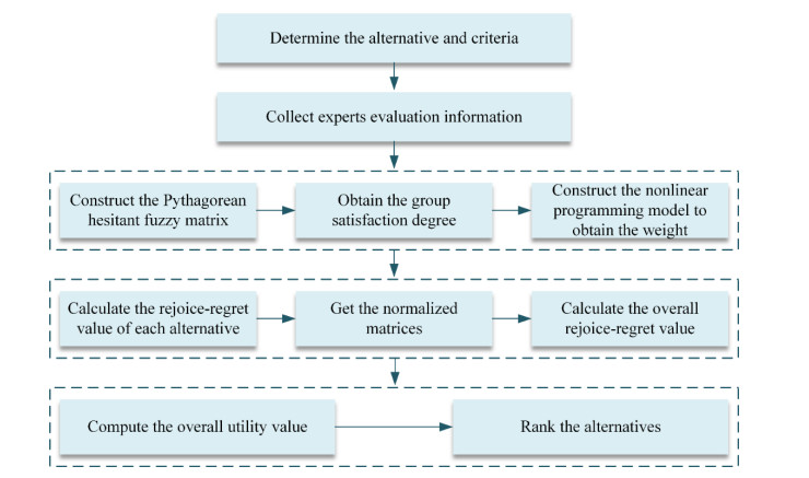
The objective of this paper is to present an extended approach to address the stochastic multi-attribute decision-making problem. The novelty of this study is to consider the regret behavior of decision makers under a Pythagorean hesitant fuzzy environment. First, the group satisfaction degree of decision-making matrices is used to consider the different preferences of decision-makers. Second, the nonlinear programming model under different statues is provided to compute the weights of attributes. Then, based on the regret theory, a regret value matrix and a rejoice value matrix are constructed. Furthermore, the feasibility and superiority of the developed approach is proven by an illustrative example of selecting an air fighter. Eventually, a comparative analysis with other methods shows the advantages of the proposed methods.

References

[1]	H. Liao, Z. Xu, Satisfaction degree based interactive decision making under hesitant fuzzy environment with incomplete weights, Int. J. Uncertainty Fuzziness Knowledge Based Syst., 22 (2014), 553–573. https://doi.org/10.1142/S0218488514500275 doi: 10.1142/S0218488514500275
[2]	M. Lin, C. Huang, R. Chen, H. Fujita, X. Wang, Directional correlation coefficient measures for Pythagorean fuzzy sets: their applications to medical diagnosis and cluster analysis, Complex Intell. Syst., 7 (2021), 1025–1043. https://doi.org/10.1007/s40747-020-00261-1 doi: 10.1007/s40747-020-00261-1
[3]	X. Gou, Z. Xu, H. Liao, Hesitant fuzzy linguistic entropy and cross-entropy measures and alternative queuing method for multiple criteria decision making, Inf. Sci., 388 (2017), 225–246. https://doi.org/10.1016/j.ins.2017.01.033 doi: 10.1016/j.ins.2017.01.033
[4]	R. Zhang, Z. Xu, X. Gou, ELECTRE Ⅱ method based on the cosine similarity to evaluate the performance of financial logistics enterprises under double hierarchy hesitant fuzzy linguistic environment, Fuzzy Optim. Dec. Making, 22 (2023), 23–49. https://doi.org/10.1007/S10700-022-09382-3 doi: 10.1007/S10700-022-09382-3
[5]	X. Gou, Z. Xu, H. Liao, F. Herrera, Probabilistic double hierarchy linguistic term set and its use in designing an improved VIKOR method: The application in smart healthcare, J. Oper. Res. Soc., 72 (2021), 2611–2630. https://doi.org/10.1007/S10700-022-09382-3 doi: 10.1007/S10700-022-09382-3
[6]	K. Atanassov, Intuitionistic fuzzy sets, Fuzzy Sets Syst., 20 (1986), 87–96. https://doi.org/10.1007/978-3-7908-1870-3_1 doi: 10.1007/978-3-7908-1870-3_1
[7]	R. R. Yager, Pythagorean membership grades in multicriteria decision making, IEEE Trans. Fuzzy Syst., 22 (2014), 958–965. https://doi.org/10.1109/TFUZZ.2013.2278989 doi: 10.1109/TFUZZ.2013.2278989
[8]	R. R. Yager, A. M. Abbasov, Pythagorean membership grades, complex numbers, and decision making, Int. J. Intell. Syst., 28 (2013), 436–452. https://doi.org/10.1002/int.21584 doi: 10.1002/int.21584
[9]	V. Torra, Hesitant fuzzy sets, Int. J. Intell. Syst., 25 (2010), 529–539. https://doi.org/10.1002/int.20418 doi: 10.1002/int.20418
[10]	M. S. A. Khan, S. Abdullah, A. Ali, N. Siddiqui, F. Amin, Pythagorean hesitant fuzzy sets and their application to group decision making with incomplete weight information, J. Intell. Fuzzy Syst., 33 (2017), 3971–3985. https://doi.org/10.3233/JIFS-17811 doi: 10.3233/JIFS-17811
[11]	S. Xian, D. Ma, H. Guo, X. Feng, Route intelligent recommendation model and algorithm under the Pythagorean hesitant fuzzy linguistic environment, Comput. Appl. Math., 42 (2023), 106–116. https://doi.org/10.1007/s40314-023-02249-2 doi: 10.1007/s40314-023-02249-2
[12]	N. Zhang, Z. Yao, Y. Zhou, G. Wei, Some new dual hesitant fuzzy linguistic operators based on Archimedean t-norm and t-conorm, Neural Comput. Appl., 31 (2019), 7017–7040. https://doi.org/10.1007/s00521-018-3534-x doi: 10.1007/s00521-018-3534-x
[13]	M. Shakeel, M. Shahzad, S. Abdullah, Pythagorean uncertain linguistic hesitant fuzzy weighted averaging operator and its application in financial group decision making, Soft Comput., 24 (2020), 1585–1597. https://doi.org/10.1007/s00500-019-03989-2 doi: 10.1007/s00500-019-03989-2
[14]	M. S. A. Khan, S. Abdullah, A. Ali, F. Amin, F. Hussain, Pythagorean hesitant fuzzy Choquet integral aggregation operators and their application to multi-attribute decision-making, Soft Comput., 23 (2019), 251–267. https://doi.org/10.1007/s00500-018-3592-0 doi: 10.1007/s00500-018-3592-0
[15]	D. Liang, Z. Xu, The new extension of TOPSIS method for multiple criteria decision making with hesitant Pythagorean fuzzy sets, Appl. Soft Comput., 60 (2017), 167–179. https://doi.org/10.1016/j.asoc.2017.06.034 doi: 10.1016/j.asoc.2017.06.034
[16]	M. S. A. Khan, S. Abdullah, A. Ali, F. Amin, An extension of VIKOR method for multi-attribute decision-making under Pythagorean hesitant fuzzy setting, Granular Comput., 4 (2019), 421–434. https://doi.org/10.1007/s41066-018-0102-9 doi: 10.1007/s41066-018-0102-9
[17]	M. F. Ak, M. Gul, AHP-TOPSIS integration extended with Pythagorean fuzzy sets for information security risk analysis, Complex Intell. Syst., 5 (2019), 113–126. https://doi.org/10.1007/s40747-018-0087-7 doi: 10.1007/s40747-018-0087-7
[18]	S. Geetha, S. Narayanamoorthy, J. V. Kureethara, D. Baleanu, D. Kang, The hesitant Pythagorean fuzzy ELECTRE Ⅲ: an adaptable recycling method for plastic materials, J. Cleaner Prod., 291 (2021), 125281. https://doi.org/10.1016/j.jclepro.2020.125281 doi: 10.1016/j.jclepro.2020.125281
[19]	R. Krishankumaar, A. R. Mishra, X. Gou, K. S. Ravichandran, New ranking model with evidence theory under probabilistic hesitant fuzzy context and unknown weights, Neural Comput. Appl., 34 (2022), 1–15. https://doi.org/10.1007/S00521-021-06653-9 doi: 10.1007/S00521-021-06653-9
[20]	J. Jana, S. K. Roy, Linguistic Pythagorean hesitant fuzzy matrix game and its application in multi-criteria decision making, Appl. Intell., 53 (2023), 1–22. https://doi.org/10.1007/S10489-022-03442-2 doi: 10.1007/S10489-022-03442-2
[21]	T. Nie, P. Liu, Z. Han, Interval neutrosophic stochastic multiple attribute decision-making method based on cumulative prospect theory and generalized shapley function, J. Intell. Fuzzy Syst., 35 (2018), 3911–3926. https://doi.org/10.3233/JIFS-18988 doi: 10.3233/JIFS-18988
[22]	X. Liu, X. Wang, L. Zhang, Q. Zeng, A novel fuzzy stochastic MAGDM method based on credibility theory and fuzzy stochastic dominance with incomplete weight information, Kybernetes, 48 (2019), 2030–2064. https://doi.org/10.1108/K-08-2018-0438 doi: 10.1108/K-08-2018-0438
[23]	G. Qu, T. Li, X. Zhao, W. Qu, Q. An, J. Yan, Dual hesitant fuzzy stochastic multiple attribute decision making method based on regret theory and group satisfaction degree, J. Intell. Fuzzy Syst., 35 (2018), 6479–6488. https://doi.org/10.3233/JIFS-18667 doi: 10.3233/JIFS-18667
[24]	G. Jiang, Z. Fan, Y. Liu, Stochastic multiple-attribute decision making method based on stochastic dominance and almost stochastic dominance rules with an application to online purchase decisions, Cognit. Comput., 11 (2019), 87–100. https://doi.org/10.1007/s12559-018-9605-6 doi: 10.1007/s12559-018-9605-6
[25]	Z. Wang, Y. Wang, Multiple attribute group decision making method based on two-dimension 2-tuple linguistic from a stochastic perspective (in Chinese), J. Syst. Sci. Math. Sci., 42 (2022), 1161–1177. https://doi.org/10.12341/jssms20411 doi: 10.12341/jssms20411
[26]	M. Rezaei, Prioritization of biodiesel development policies under hybrid uncertainties: A possibilistic stochastic multi-attribute decision-making approach, Energy, 260 (2022), 125074–125086. https://doi.org/10.1016/J.ENERGY.2022.125074 doi: 10.1016/J.ENERGY.2022.125074
[27]	D. E. Bell, Regret in decision making under uncertainty, Oper. Res., 30 (1982), 961–981. https://doi.org/10.1287/opre.30.5.961 doi: 10.1287/opre.30.5.961
[28]	G. Loomes, R. Sugden, Regret theory: An alternative theory of rational choice under uncertainty, Econ. J., 92 (1982), 805–824. https://doi.org/10.2307/2232669 doi: 10.2307/2232669
[29]	J. Quiggin, Regret theory with general choice sets, J. Risk Uncertainty, 8 (1994), 153–165. https://doi.org/10.1007/BF01065370 doi: 10.1007/BF01065370
[30]	X. Liu, J. Zhu, S. Zhang, S. Liu, Hesitant fuzzy stochastic multiple attribute decision making method based on regret theory and group satisfaction degree (in Chinese), Chin. J. Manage. Sci., 25 (2017), 171–178. https://doi.org/10.16381/j.cnki.issn1003-207x.2017.10.018 doi: 10.16381/j.cnki.issn1003-207x.2017.10.018
[31]	L. Zhu, Hesitant fuzzy decision-making method based on regret theory and evidence theory (in Chinese), J. Comput. Appl., 37 (2017), 540–545 + 568. https://doi.org/10.11772/j.issn.1001-9081.2017.02.0540 doi: 10.11772/j.issn.1001-9081.2017.02.0540
[32]	L. Wei, Y. Wang, Interval-valued hesitant fuzzy stochastic decision-making method based on regret theory, Int. J. Fuzzy Syst., 22 (2020), 1091–1103. https://doi.org/10.1007/s40815-020-00830-z doi: 10.1007/s40815-020-00830-z
[33]	X. Tian, Z. Xu, G. Jing, F. Herrera, A consensus process based on regret theory with probabilistic linguistic term sets and its application in venture capital, Inf. Sci., 562 (2021), 347–369. https://doi.org/10.1016/j.ins.2021.02.003 doi: 10.1016/j.ins.2021.02.003
[34]	X. Jia, X. Wang, A PROMETHEE Ⅱ method based on regret theory under the probabilistic linguistic environment, IEEE Access, 8 (2020), 228255–228263. https://doi.org/10.1109/ACCESS.2020.3042668 doi: 10.1109/ACCESS.2020.3042668
[35]	J. Ali, Z. Bashir, T. Rashid, W. K. Mashwani, A q-rung orthopair hesitant fuzzy stochastic method based on regret theory with unknown weight information, J. Ambient Intell. Hum. Comput., 1 (2022), 1–18. https://doi.org/10.1007/S12652-022-03746-8 doi: 10.1007/S12652-022-03746-8
[36]	J. Zhu, X. Ma, J. Zhan, Y. Yao, A three-way multi-attribute decision making method based on regret theory and its application to medical data in fuzzy environments, Appl. Soft Comput., 123 (2022), 108975–109003. https://doi.org/10.1016/J.ASOC.2022.108975 doi: 10.1016/J.ASOC.2022.108975
[37]	J. Liu, L. Shao, F. Jin, Z. Tao, A multi-attribute group decision-making method based on trust relationship and DEA regret cross-efficiency, IEEE Trans. Eng. Manage., 2022 (2022), 1–13. https://doi.org/10.1109/TEM.2021.3138970 doi: 10.1109/TEM.2021.3138970
[38]	H. Liao, Z. Xu, Satisfaction degree based interactive decision making under hesitant fuzzy environment with incomplete weights, Int. J. Uncertainty Fuzziness Knowledge Based Syst., 22 (2014), 553–573. https://doi.org/10.1142/S0218488514500275 doi: 10.1142/S0218488514500275
[39]	D. F. Li, G. H. Chen, Z. G. Huang, Linear programming method for multiattribute group decision making using IF sets, Inf. Sci., 180 (2010), 1591–1609. https://doi.org/10.1016/j.ins.2010.01.017 doi: 10.1016/j.ins.2010.01.017
[40]	M. Sajjad Ali Khan, A. Ali, S. Abdullah, F. Amin, F. Hussain, New extension of TOPSIS method based on Pythagorean hesitant fuzzy sets with incomplete weight information, J. Intell. Fuzzy Syst., 35 (2018), 5435–5448. https://doi.org/10.3233/JIFS-171190 doi: 10.3233/JIFS-171190
[41]	L. A. Zadeh, The concept of a linguistic variable and its application to approximate reasoning-I, Inf. Sci., 8 (1975), 199–249. https://doi.org/10.1016/0020-0255(75)90036-5 doi: 10.1016/0020-0255(75)90036-5
[42]	D. Liu, Y. Liu, X. Chen, Fermatean fuzzy linguistic set and its application in multicriteria decision making, Int. J. Intell. Syst., 34 (2019), 878–894. https://doi.org/10.1002/int.22079 doi: 10.1002/int.22079

Reader Comments

Your name:*

Email:*
© 2023 the Author(s), licensee AIMS Press. This is an open access article distributed under the terms of the Creative Commons Attribution License (http://creativecommons.org/licenses/by/4.0)